How to Filter Merged Cells in Excel

This tutorial demonstrates how to filter merged cells in Excel.

 

 

Filter Merged Cells

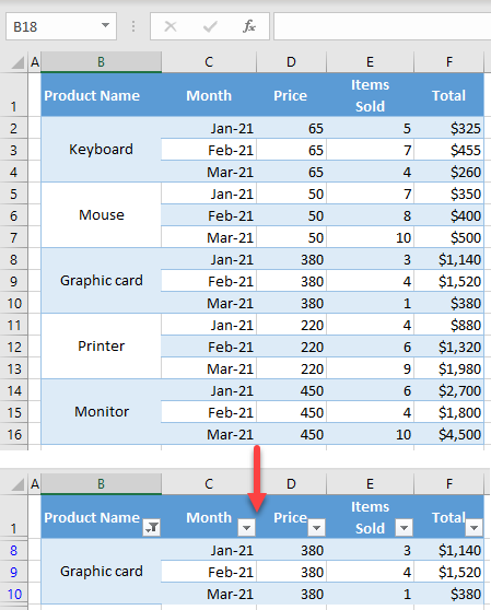
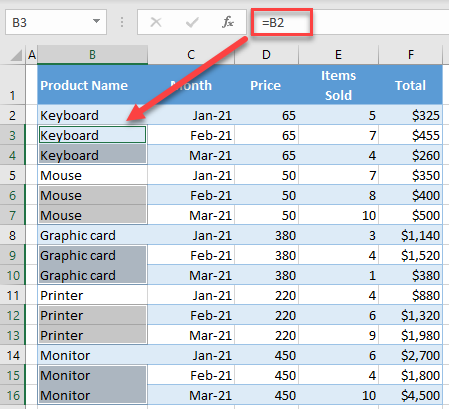
When you filter a data set that has merged cells across rows, Excel returns only the first row of the merged cells. Say you have the following data set.

 

 

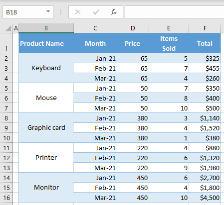
As you can see, product names in Column B are merged across three rows to display three months of data (cells B2: B4 are merged, B5:B7, etc.). If you know want to filter for graphic card and display data for this product only, Excel displays only Row 8, the first row containing graphic card in Column B.

 

 

This happens because while filtering, Excel unmerges all cells by default and considers, in this case, B9 and B10 to be blank. To see all relevant rows (8–10) when filtering for graphic card, follow these steps:

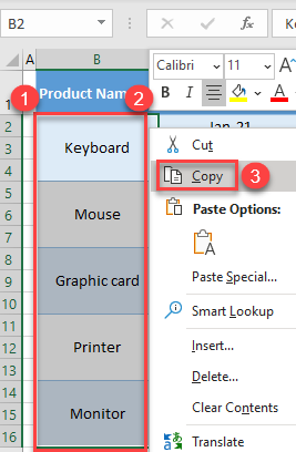
1. First, copy the data to another location.
   Select the range with merged cells (B2:B16), right-click the selected area, and choose Copy (or use the keyboard shortcut CTRL + C).

 

 

2. Right-click outside the data set (e.g., H2) and choose Paste (or use the keyboard shortcut CTRL + V).

 

 

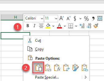
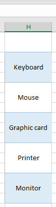
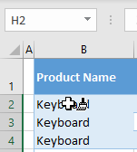
As a result of Steps 1 and 2, the merged cells from Column B, are now copied to Column H, with the same formatting. This range will later be copied back to the data set.

 

 

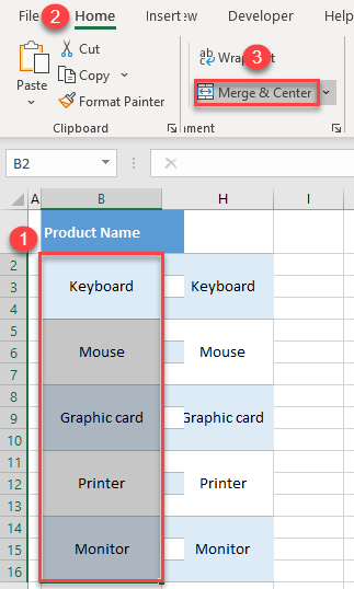
3. Now unmerge all cells, and populate blank cells with the appropriate product names.
   Select the range of merged cells in Column B (B2:B16), and in the in Ribbon, go to Home > Merge & Center.

 

 

4. Keep the same range selected (B2:B16), and in the Ribbon, go to Home > Find & Select > Go To Special…

 

 

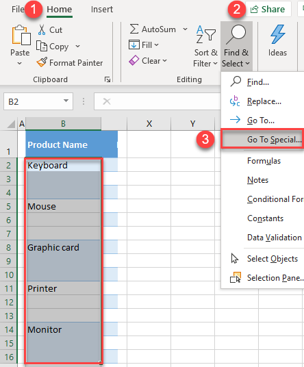
5. In the Go To Special window, select Blanks and click OK.

 

 

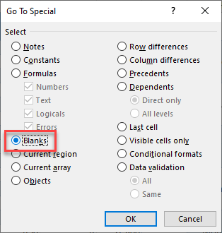
6. Now all blank cells are selected.
   In cell B3, type “=B2” (to copy the value from cell B2), and press CTRL + ENTER on the keyboard.
   This populates the formula in the selected range: All blank cells are populated with the appropriate product name.

 

 

7. Now, use the copied column (H) to return Column B to its original format.
   Select the previously copied merged cells from Column H, and in the Ribbon, go to Home > Format Painter.

 

 

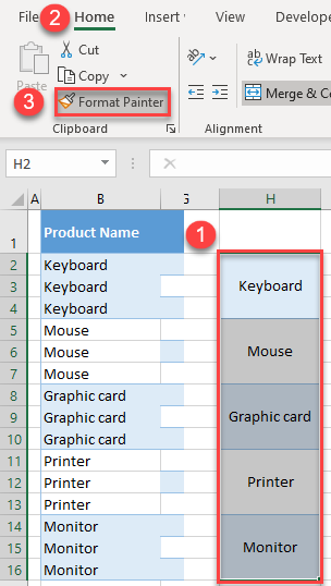
8. Click on the first cell in the range (B2), to paste formats.

 

 

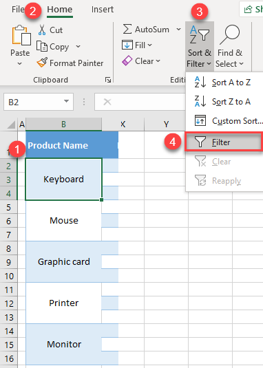
9. You can now filter data in Column B. First, turn on the filter.
   Click anywhere in the data range, and in the Ribbon, go to Home > Sort & Filter > Filter.

 

 

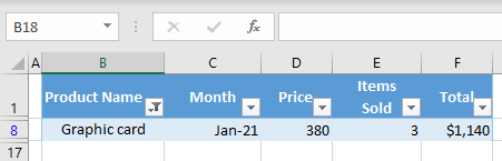
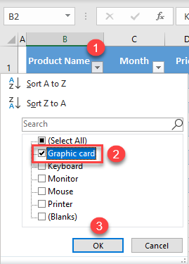
10. Click on the filter icon for Column B (the arrow in cell B1). Uncheck (Select All) and select only graphic card.

 

 

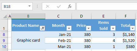
As a result, all three rows of graphic card (8–10) are filtered, showing that merged cells are filtered successfully.

 

 

See our VBA tutorials to see how to work with filters and merging cells within a macro.