How to Hide Blank Rows in Excel & Google Sheets

This tutorial demonstrates how to hide blank rows in Excel and Google Sheets.

Filter to Hide Blank Rows

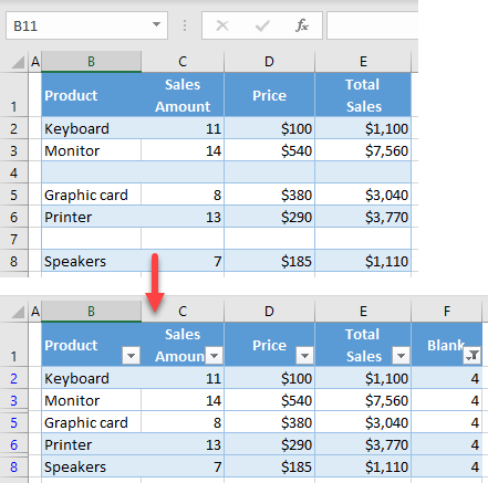
You can hide blank rows using filters and a helper column. Say you have the following data set.

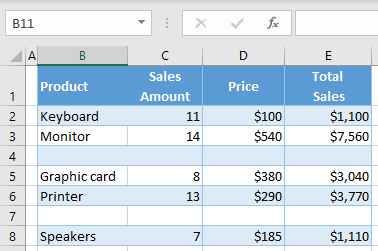
You want to hide Rows 4 and 7, as they are completely blank. First, you need a helper column to indicate if a row is blank using the COUNTA Function.

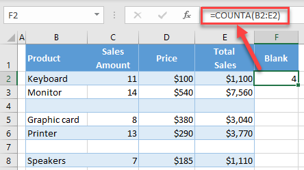
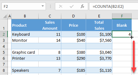
1. Add a new column (F) to serve as a helper column for filtering blank rows. In cell F2, enter the formula:

=COUNTA(B2:E2)

This formula returns the number of non-blank cells in the given range (in this case, in B2:E2). If you get a zero in any cell, that means the row is blank, because there are no non-blank values.

2. Now position the cursor in the bottom right corner of cell F2 until a black cross appears and drag it through the last row of the data range (Row 8).

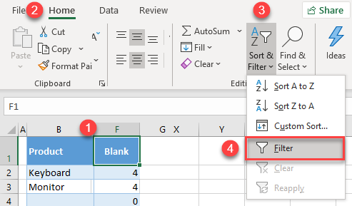
3. Now the formula is in the range F2:F8. Filter out all zero values to hide blank rows. First, turn on the filter for Column F (Blank). Select any cell in the column (in this case, F1), and in the Ribbon, go to Home > Sort & Filter > Filter.

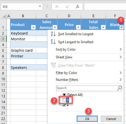
4. To filter out blank (zero) values, click on the filter icon in the F1 cell, uncheck 0, and click OK.

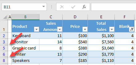
As a result, all blank rows (in this case 4 and 7) are hidden. Note that that rows numbers are blue and hidden rows heading are missing. This shows that some rows in the worksheet are hidden.

Note: You can also use VBA code to hide or delete blank rows.

Hide Blank Rows in Google Sheets

You can also hide all blank rows in Google Sheets.

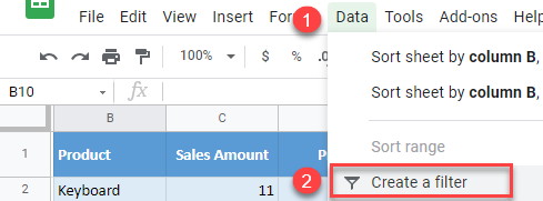
1. Once you insert the formula (=COUNTA(B2:E2)) in Column F, turn on the filter by going to Data > Create a filter.

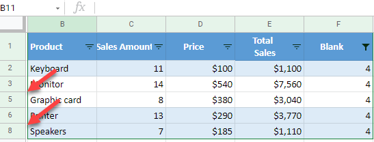
2. To filter out zero values, click on the filter icon in the F1 cell, uncheck 0, and click OK.

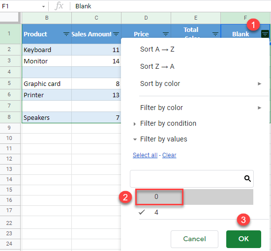
All blank rows are now hidden.