How to Highlight Multiple Rows in Excel & Google Sheets

This tutorial demonstrates how to highlight multiple rows in Excel and Google Sheets.

 

 

Highlight Adjacent Rows

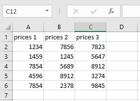
Say you have a data set with prices and you want to highlight Rows 3, 4, and 5.

 

 

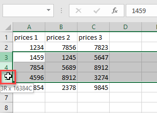
1. To select rows, select the first one (Row 3) by clicking on the row number and drag the cursor to the last row you want (Row 5).

 

 

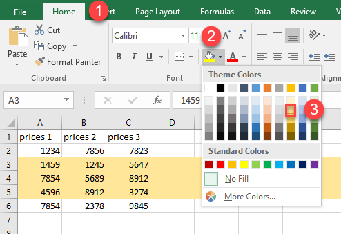
2. Now, highlight the rows you selected in Step 1. In the Ribbon, go to the Home tab, click on the Fill Color icon, and choose the color.

 

 

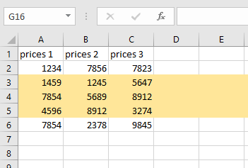
As a result, the selected rows are highlighted.

 

 

Highlight Non-Adjacent Rows

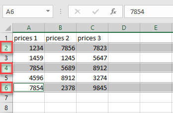
Suppose you have the same data set, and you want to highlight non-adjacent rows (Rows 2, 4, and 6).

 

 

1. Select the first row you want to highlight (Row 2), hold the CTRL key, and click on the numbers of each other row you want to highlight (Rows 4 and 6).

 

 

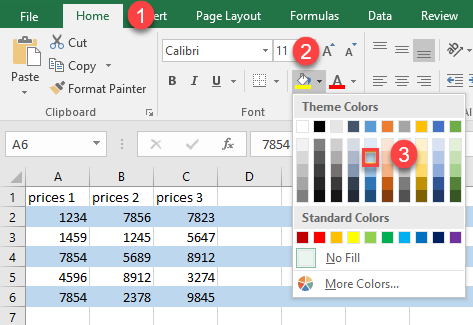
2. To highlight selected rows, in the Ribbon go to Home, click on the Fill Color icon, and choose the color from the pallet.

 

 

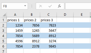
After that, all selected rows are highlighted.

 

 

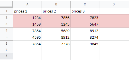
Highlight Rows in Google Sheets

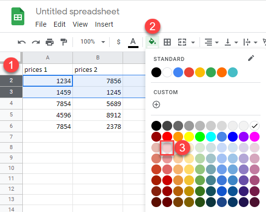
1. Select adjacent rows by selecting the first one and dragging the cursor to the last row you want to highlight (here, Rows 2 and 3).
2. In the Toolbar, click on the Fill color icon.
3. Then choose a color from the palette.

 

 

As a result, the selected rows are highlighted.

 

 

The process of highlighting non-adjacent rows in Google Sheets is the same as it is in Excel.