How to Make a Pivot Table Chart in Excel & Google Sheets

This tutorial demonstrates how to make a pivot table chart in Excel and Google Sheets.

 

 

Create Pivot Chart

A pivot chart is similar to a chart created from a data table, except that it is based specifically on a pivot table.

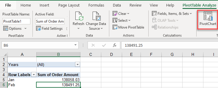
1. Click in your pivot table, and then in the Ribbon, go to PivotTable Analyze > Pivot Chart.

 

 

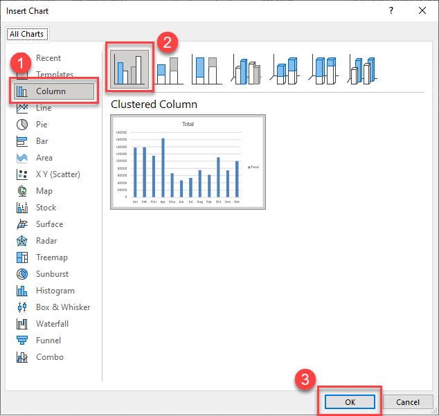
2. Choose the type of chart you wish to create (column, line, bar, etc.), and then choose from the chart styles (e.g., Clustered Column) for that type of chart. To insert the chart into the worksheet, click OK.

 

 

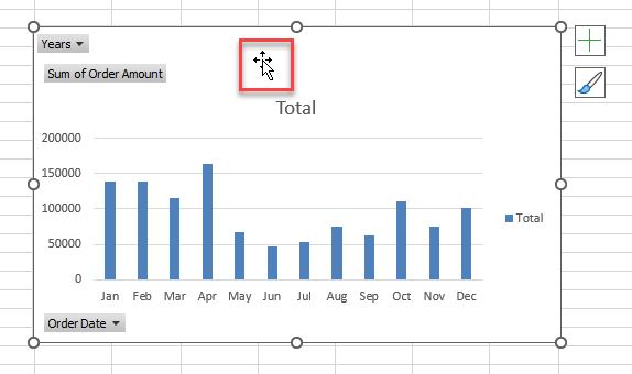
3. To move the chart, click somewhere in the middle of the chart – your mouse should have a small black cross attached to it – and drag to the desired location.

 

 

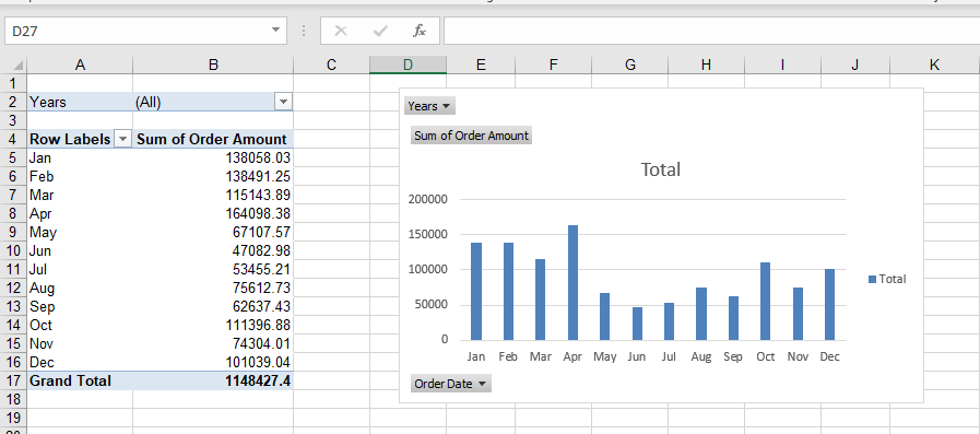
Drill Down in a Pivot Chart

The chart displays all the information that is shown in the pivot table. You can filter (drill down) either in the pivot table or in the pivot chart.

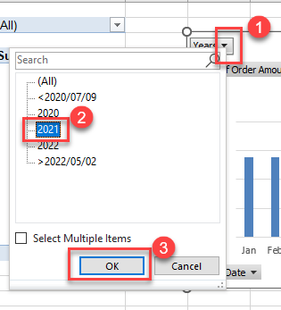
1. For this example, click the arrow to the right of the filter field (years), to drill down to a specific year.
2. Click on the value you want (2021).
3. Click OK.

 

 

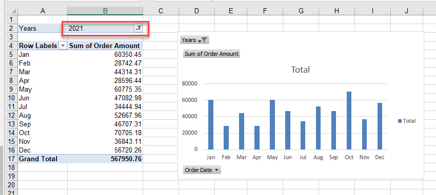
The data in both the pivot chart and the pivot table is filtered to show just the year you chose.

 

 

Change Chart Type

1. Click in your chart, and then, in the Ribbon, go to Design > Change Chart Type.

 

 

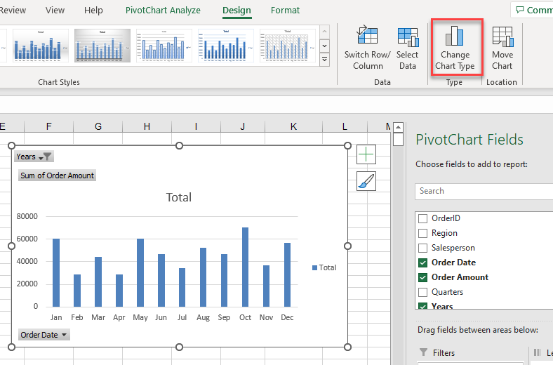
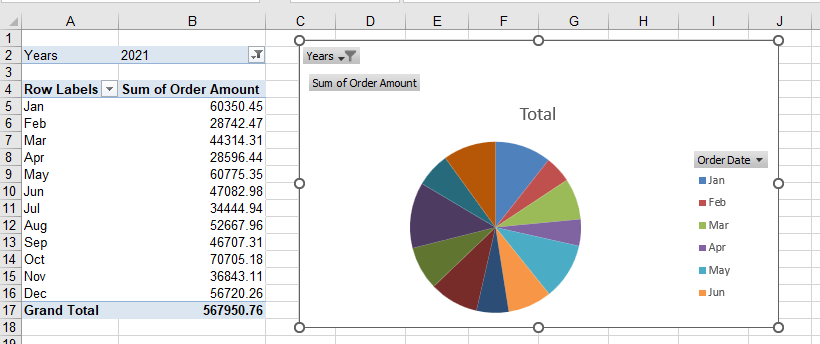
2. Choose from the chart types, and then click OK.

 

 

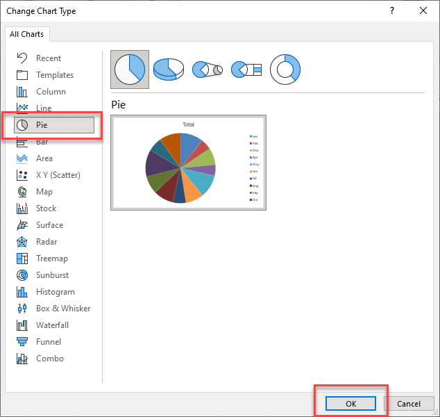
3. Confirm that the updated chart looks how you wanted or go back to Step 1 to try something else.

 

 

Print Pivot Chart

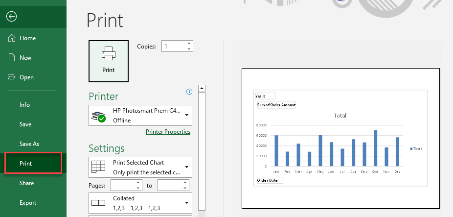
To print just the pivot chart – excluding the pivot table – click just on the chart and in the Ribbon, go to File > Print.

 

 

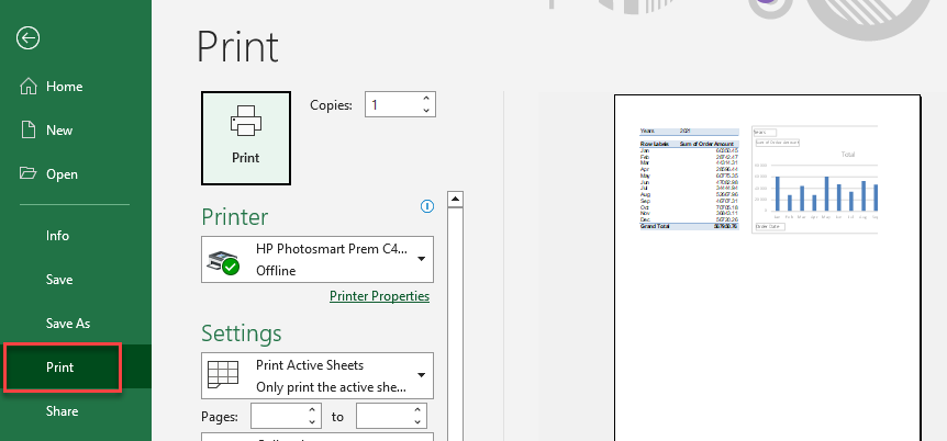
To print the sheet showing both the pivot table and the chart (and other content, if applicable), click off the chart so that a cell in the worksheet is selected. Then in the Ribbon, go to File > Print.

 

 

Tip: Try using some shortcuts when you’re working with pivot tables.

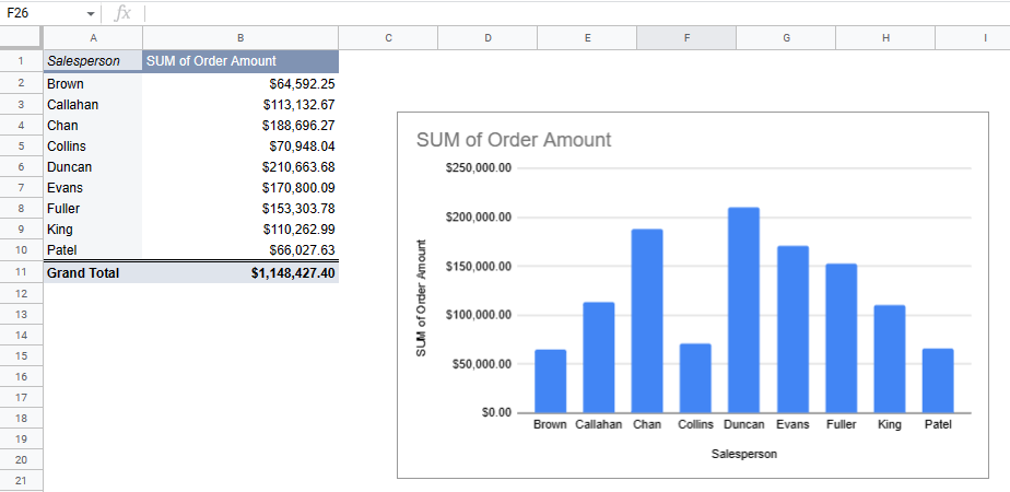
Pivot Table Chart in Google Sheets

Once you have set up a pivot table in Google Sheets, you can insert a chart based on the data in the table.

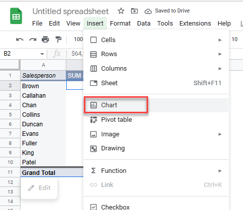
1. Click in your pivot table, and then in the Menu, go to Insert > Chart.

 

 

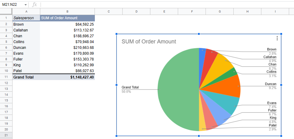
2. This automatically creates a chart for you.

 

 

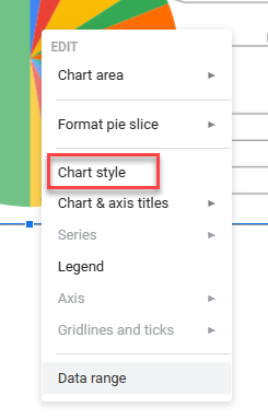
3. Right-click on the chart, then click Chart style.

 

 

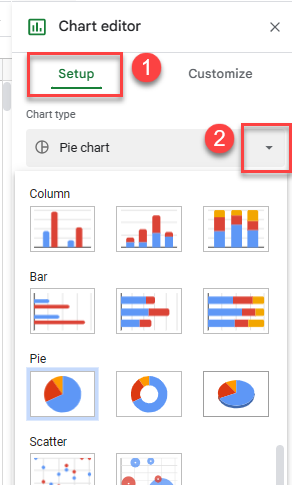
4. Click on the Setup tab, and then choose from the chart types in the drop down.

 

 

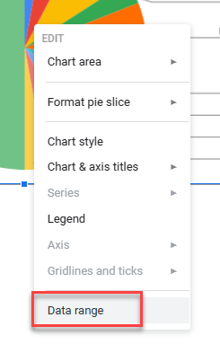
5. To change the data range (e.g., if you don’t want the total line of the pivot table included), right-click once again on the chart, and then click Data Range.

 

 

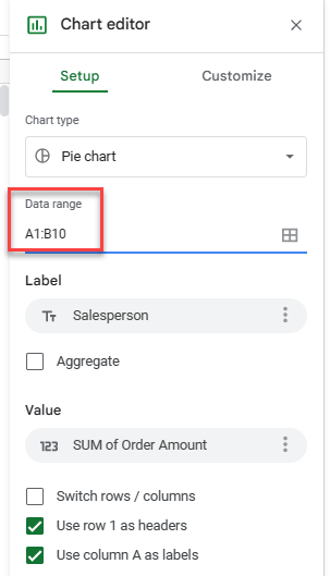
6. Adjust the data range as necessary. (Here, the range is changed to exclude Row 11.)

 

 

7. Your chart is adjusted to show the new style and range. Confirm it looks how you wanted it to, or go back to Step 3 to try something else.