How to Reverse the Order of Data in Excel & Google Sheets
Written by
Reviewed by
In this tutorial, you will learn how to reverse the order of data in Excel and Google Sheets.
Reverse the Order of Data
Use Helper Column and Sort
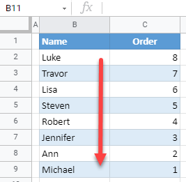
There are several ways to reverse the order of data (flip it “upside down”) in Excel. The following example uses a helper column that will then be sorted. Say you have the list of names below in Column B and want to sort it in reverse order.
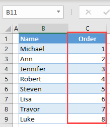
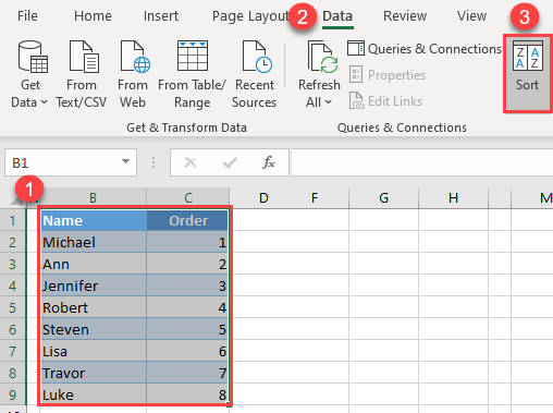
- In Column C, add serial numbers next to the names in Column B. Start at 1 and increase by 1 for each name. Column C is the helper column you’ll use to sort the data in reverse order by going from ascending to descending.
- Select the entire data range (B1:B9), and in the Ribbon, go to Data > Sort.
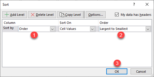
- In the Sort window, (1) select Order for Sort by, (2) Largest to Smallest for Order, and (3) click OK.
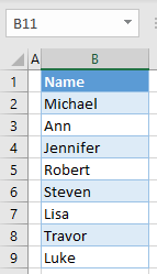
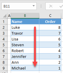
As a result, the data range is sorted in a descending order by Column C, which means that names in Column B are now in the reverse order. You can delete the helper column now.
Reverse Order With a Formula
Another way to reverse the data order is to use the INDEX and ROWS Functions.
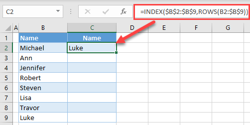
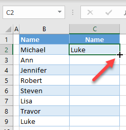
- Enter the following formula in cell C2:
=INDEX($B$2:$B$9,ROWS(B2:$B$9))Let’s walk through how this formula works:
-
- The INDEX Function takes a data range (the first parameter) and a row (the second parameter) and returns a value. In this case, the range is always B2:B9, and the row is the output of the ROWS Function.
- The ROWS Function in this example returns the number of rows in the selected range, which starts at the current row and ends at the last cell.
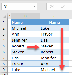
So for cell C2, the result of the ROWS Function is 8 (There are eight rows from B2 through B9.), so the INDEX Function will return the value in the eigth row of the data range, which is Luke. For cell C3, the result of the ROWS Function is 7 (There are seven rows from B3 through B9.), so the INDEX Function returns Travor. In this way, the row for the INDEX Function will decrease by one each time and form the original list in reverse order.
- Position the cursor in the bottom right corner of cell C2 until the cross appears, then drag it down through Row 9.
The final result is the data set from Column B sorted in reverse order in Column C.
Reverse Data Order in Google Sheets
In Google Sheets, you can use the INDEX and ROWS formula exactly the same as in Excel. But the helper column method works a bit differently
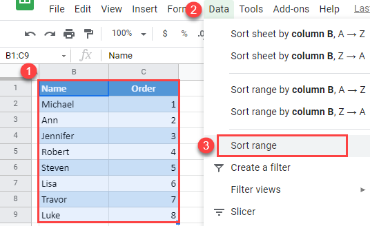
- Select the entire data range, including the helper column (B1:C9) and in the Menu, go to Data > Sort range.
- In the Sort window, (1) check Data has header row, (2) choose Order for Sort by, (3) select Z → A (descending), and (4) click Sort.
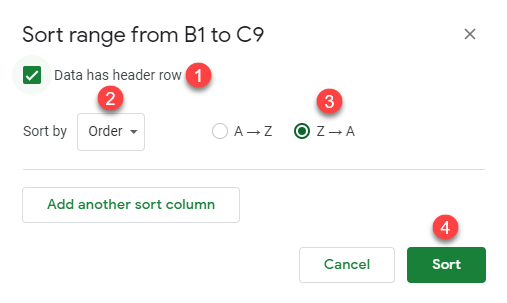
As a result, the names are now in the reverse order in Column C.