This tutorial will demonstrate how to test if data is normally distributed (normality) in Excel and Google Sheets.

How to Perform a Test For Normality in Excel

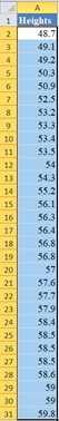
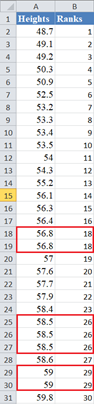
Background: A sample of the heights, in inches, of 30 ten years old boys are presented in the table below. Using the graphical methods of test for normality, test whether the data obtained from the sample can be modeled using a normal distribution.

Histogram Method

A histogram is a graphical representation of the frequency/probability distribution of continuous data. The frequency distribution is represented with rectangles whose heights correspond to the frequency of each class and the width represents the class intervals/boundaries.

To test for normality using a histogram, you compare the histogram of the data set to the normal probability curve. If the histogram is approximately bell-shaped, you can assume that the data set is normally distributed.

First, we group the data set into classes. You can determine the number of classes you want to group the data or you can use the Sturges rule for determining the number of classes (n) in a data set of size N given by n=1+3.3 log⁡N.

Using the Sturges rule for our data set, we have that the desired number of classes for our data set which has 30 data points is 6 groups. Then, we obtain the width of each group by subtracting the minimum data point from the maximum data point and dividing the result by 6 groups.

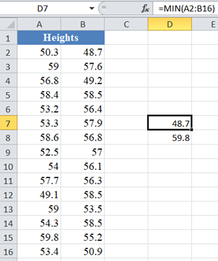
Using the Min and Max Functions, we get that the minimum data point and the maximum data point are 48.7 and 59.8 respectively.

Thus, the class width is (59.8-48.7)/6=1.85 , but for convenience, we approximate the class width to 2 and extend the minimum and the maximum to 48 and 60 respectively. Then we have the class intervals as follows:

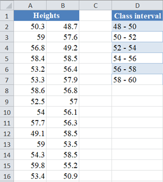
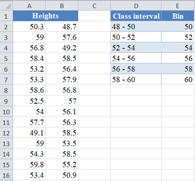
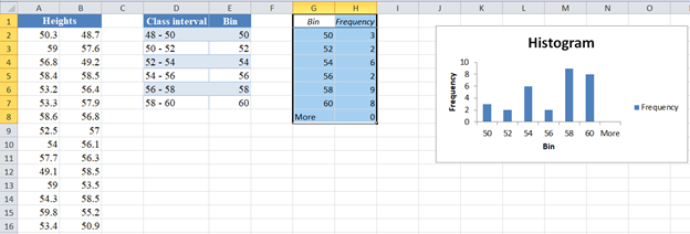
Next, to construct a histogram in Excel we need to have the ‘Bin’ column, the Bin represents the upper bound of the class intervals. So, we have the Bin column as follows:

Next, construct the histogram of the data.

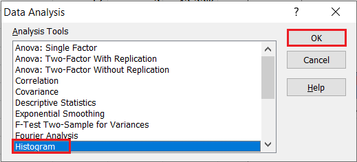
Use the “Histogram” feature located in the Data Ribbon > Data Analysis.

If you don’t see the Data Analysis option, you will need to install the Data Analysis Toolpak.

In the Data Analysis window, choose Histogram and click OK.

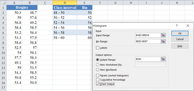
Configure the parameters as follows.

• Click on “Input Range” and select the cells containing the source data.
• Click on “Bin Range” and select the cells containing the bins.
• Select the “Labels in first row” checkbox if the selected range contains column headers. Here, we did not include the headers, hence we did not select the “Labels in first row” checkbox.
• Select the desired output option. To get the results on the same sheet, select the Output range and specify the specific reference to the cell into which to display the matrix. In our case, it is $G$1
• For effective result in determining the shape of the distribution using histogram, do not set the “Pareto (sorted histogram)” and the “Cumulative Percentage” checkboxes.
• Finally, select the “Chart Output” checkbox in other to display the histogram.

The output for the Histogram is as follows:

To make the chart look more like a histogram, we make some adjustments to the chart as follows:

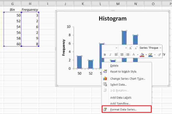
• First, delete the “More” row from the “Bin/Frequency” table.
• Next, right-click any of the rectangles and select the “Format Data Series…” option.

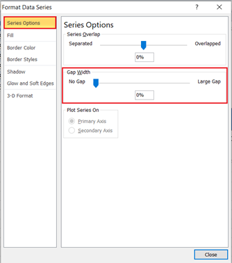
• On the “Series Options” option, move the slider in the “Gap Width” section to the “No Gap” side or enter “0%” in the box in the “Gap Width” section.

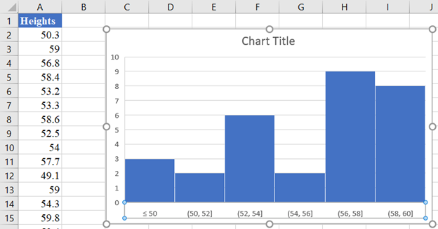
Thus, we have the final output of the histogram as follows:

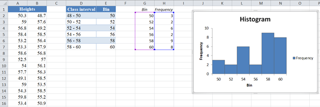
Clearly, you can see that the histogram is neither bell-shaped nor symmetric about the center. So, we can conclude that the given data cannot be modeled by a normal distribution.

Alternatively, if you use Excel 2016 or later or the Microsoft 365 packages, you can create a histogram through Insert > Insert Statistic Chart > Histogram.

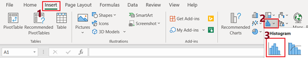
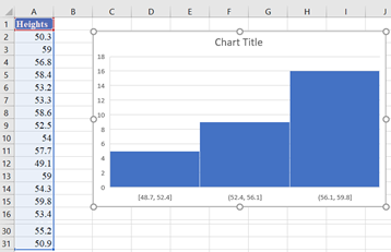
Place the dataset in one column, select the data together with the label and then click Insert > Insert Statistic Chart > Histogram. In our case we have the following output:

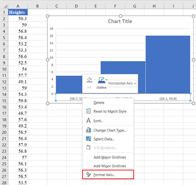
Next, adjust the chart to your preferences by configuring the number of bins and bin width. Right-click on the horizontal axis and click Format Axis:

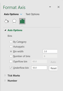
On the Axis Options option, set the Bin width or the Number of bins radio button, set the Overflow bin, and/or the Underflow bin. Overflow bin is a point in the dataset where all values greater than that point are grouped in one bin while Underflow bin is a point where all values smaller than the point are grouped in one bin.

In our case, we set the bin width to 2 and the Underflow bin to 50 as shown below:

The adjusted chart is shown below:

Boxplot Method

A boxplot is a graph of the five-number summary of a dataset. It shows the minimum and the maximum values, the first and the third quartile, and the median. The median is represented by a line that divides a rectangle into two portions. The parallel edges of the rectangle represent the first and the third quartile. Perpendicular lines (called the whiskers) are drawn from the quartiles to the minimum and the maximum values.

For normally distributed data, the median line of the boxplot will be located at approximately the center of the rectangle while the two whiskers will be approximately equal in length. Thus, a dataset that meets the above conditions can be assumed to be normally distributed; otherwise, the data is not normally distributed.

Excel versions prior to 2016 do not have the boxplot chart included among its chart templates. However, there is a workaround which I will show you in this article. I will also show you how to plot the boxplot using the boxplot chart template in Excel 2016 and later packages.

In the following steps, I will show you how to plot the boxplot in Excel versions earlier than 2016 using the boys’ heights example above.

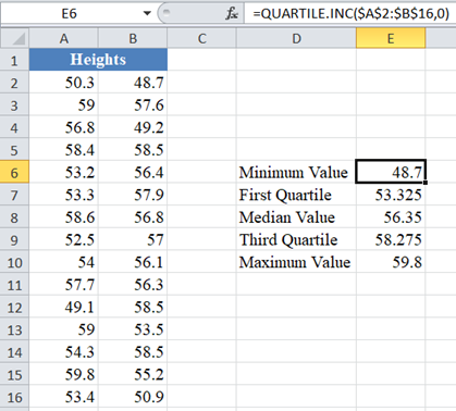
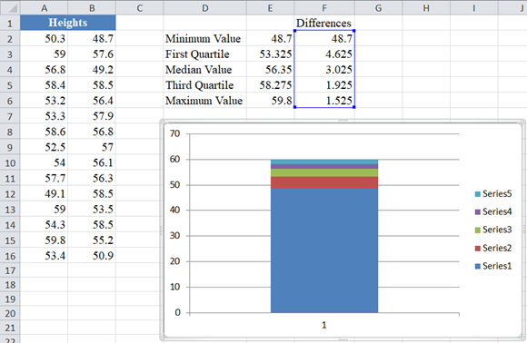
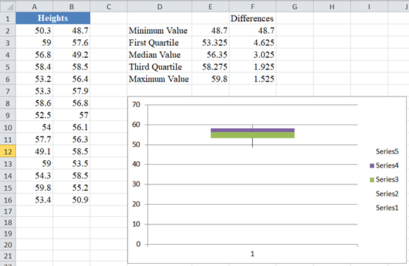
First, calculate the quartile values from the dataset using the QUARTILE.INC Function with ‘quart’ values: 0 for the minimum value, 1 for the first quartile, 2 for the median, 3 for the third quartile, and 4 for the maximum value, as shown below:

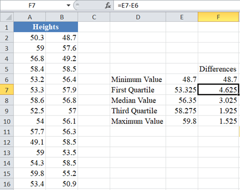
Next, calculate the differences between each quartile value with the preceding quartile value, keeping the minimum value constant. That is, create a column called “Differences” which will contain the minimum value in its first row, First Quartile – Minimum Value in the second row, Median Value – First Quartile, Third Quartile – Median Value, and Maximum Value – Third Quartile in the third, fourth, and fifth rows as shown below:

Next, create a stacked column chart through Insert > Insert Column Chart > Stacked Column using the “Differences” column.

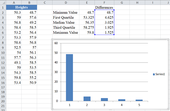
Next, reverse the chart axes by right-clicking on the chart and clicking Select Data > Switch Row/Column, and then click OK.

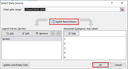
The chart then changes to:

Next, convert the chart to a boxplot following the steps below:

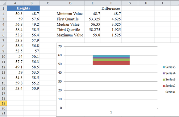
• Hide the bottom data series by right-clicking on the bottom part of the column chart and clicking on Format Data Series…, on the Fill tab, select No Fill and then close the pop-up box.

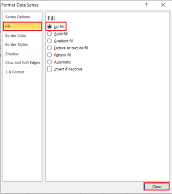
The chart then becomes:

• Create whiskers for the boxplot by replacing the topmost and the now bottom colored part of the column chart to line (or whiskers). Right-click on the topmost part of the column chart and click on Format Data Series…, on the Fill tab, select No Fill, and then close the pop-up box. Then from the ribbon, click Design > Add Chart Element > Error Bars > Standard Deviation, or on the Chart Tools section of the ribbon click Layout > Error Bars > Error bars with Standard Deviation.

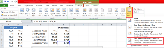
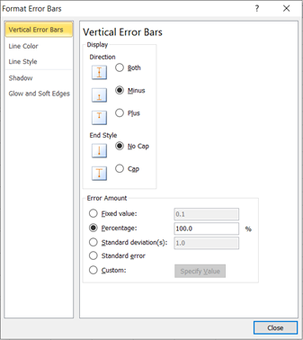
Still on Layout > Error bars, select More Error Bars Options. In the Vertical Error Bars option, set Direction to Minus, set End Style to No Cap, and set Error Amount to 100.

Repeat the above steps for the second from the bottom data series (the now bottom colored part).

The chart then becomes:

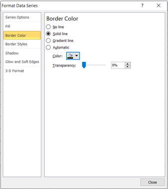
• Finally, we format the middle area as follows: Right-click the top colored part of the boxplot and click on Format Data Series…, on the Fill tab, select No Fill and on the Border Color tab, select Solid line, then set the Color to Black and close the pop-up box.

Repeat the above step for the last colored part. You can also format the axis by adjusting the ranges so that the boxplot looks bigger and better. The chart now looks like this:

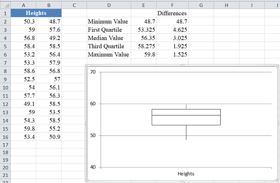
From the boxplot, you can observe that line divided the rectangle into two portions such that the bottom part of the rectangle is bigger than the top portion. Also, the bottom whisker is longer than the top whisker. Hence, we can conclude that the dataset does not represent normally distributed data.

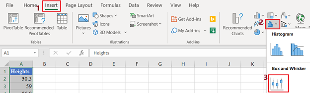
Alternatively, if you use Excel 2016 or later or the Microsoft 365 packages, you can create a boxplot by selecting the dataset and clicking Insert > Insert Statistic Chart > Box and Whisker.

The output is shown below:

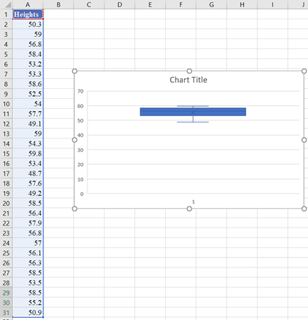
You can then format the axis to make the boxplot look bigger and clearer to your preferences.

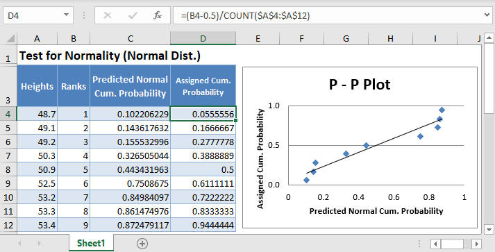
P-P Plot Method

A P–P plot (short for probability – probability plot or percent – percent plot) is a graph used to determine whether a given dataset fits a specific probability distribution. To test for normality using a normal P–P plot, you plot the cumulative probabilities of the rank of the values of the dataset against their corresponding probabilities of the values predicted by the normal distribution. If the resulting graph is approximately a straight line, the dataset can be assumed to be normally distributed; otherwise, the dataset is not normally distributed.

In the following steps, I will show you how to plot a normal probability P–P plot using the boys’ heights example above.

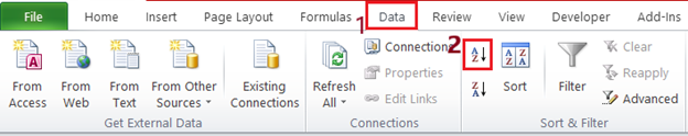
First, place the dataset in one column, select the values in the dataset and Sort the data: Data > Sort (Sort Smallest to Largest) to arrange the values in ascending order as shown below:

And the arranged values are as follows:

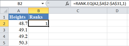
Next, use the RANK.EQ Function to obtain the ranks of the values in the dataset as follows.

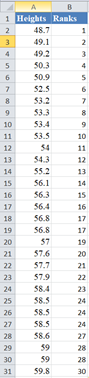
Complete the ranks of other values in the dataset.

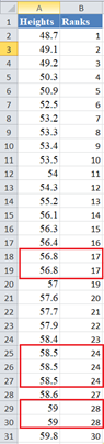
The RANK.EQ Function returns the top rank of a set of values that has the same rank; however, for the purpose of this plot, we will need the bottom ranks instead. So, we will manually change the ranks of the set of values having the same rank. Thus, we change the following ranks:

to:

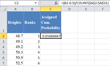
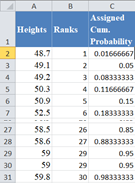
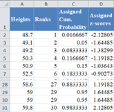
Next, calculate the cumulative probability of the ranks of the dataset. We will use the formula:

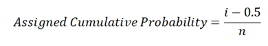
where i is the rank and  n is the size (count) of the dataset. Thus, we have:

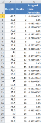
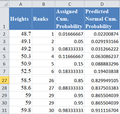
Complete the rest of the assigned cumulative probability as shown below:

Next, calculate the normal predicted cumulative probability for the dataset using the NORM.DIST Function. x is the value from the dataset,  is the average of the dataset, and  is the standard deviation of the dataset and cumulative is TRUE. Thus, we have:

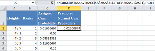
Complete the rest of the predicted normal cumulative probability as shown below:

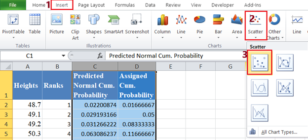
Finally, plot a scatter plot with the Predicted Normal Cumulative Probability on the x-axis and the Assigned Cumulative Probability on the y-axis. I will have to swap the positions of the Predicted Normal Cum. Probability and the Assigned Cum. Probability columns so that the Predicted Normal Cum. Probability comes first. Select the two columns with the labels and click Insert > Scatter > Scatter with only Markers as shown below:

And we get the following graph:

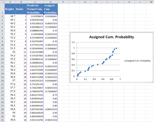
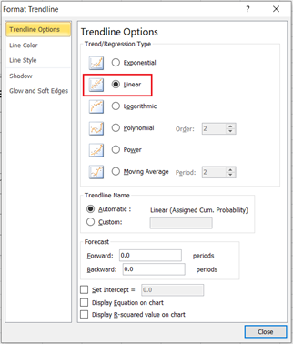
Then, add the trend line to the graph by right-clicking on any of the data points on the graph and selecting Add Trendline. On the Trendline Options, make sure that the Trend/Regression Type is set as Linear, then close the box.

You can also make some other adjustments to the graph like adding the axis’ names and editing the title, etc. Thus, we have the output as shown below:

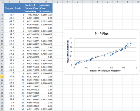
From the P–P plot, we can see that a lot of the data points digress significantly from the trend line, hence we can conclude that the data is not normally distributed.

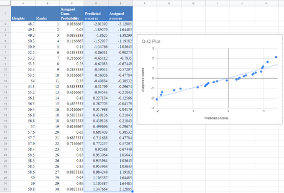
Using the Q-Q Plot

A Q–Q plot (short for quantile – quantile plot) is a graph used to determine whether a given dataset fits a specific probability distribution. The Q–Q is similar to the P–P plot except that in Q–Q, you plot the quantiles of the dataset against their corresponding quantile predicted by the normal distribution. If the resulting graph is approximately a straight line, the dataset can be assumed to be normally distributed; otherwise, the dataset is not normally distributed.

In the following steps, I will show you how to plot a normal probability Q–Q plot using the boys’ heights example above.

First, follow the steps as described in the P–P plot section to obtain up to the assigned cumulative probability of the dataset as shown below:

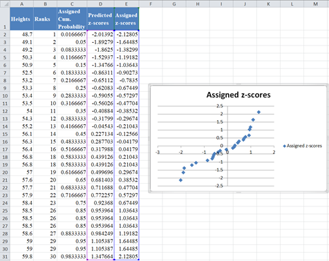
Next, calculate the z-score that corresponds to each of the assigned cumulative probability using the NORM.S.INV Function, where  is the assigned cumulative probability value. Thus, we have:

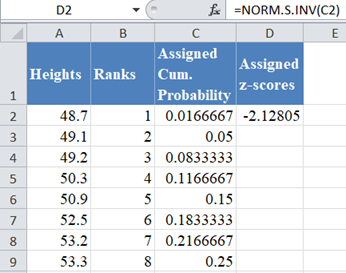
Complete the rest of the assigned z-scores column as shown below:

Next, calculate the normal predicted z-scores for the dataset using the formula

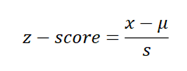
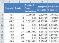
where x is the value from the dataset, μ is the average of the dataset, and s is the standard deviation of the dataset. Thus, we have:

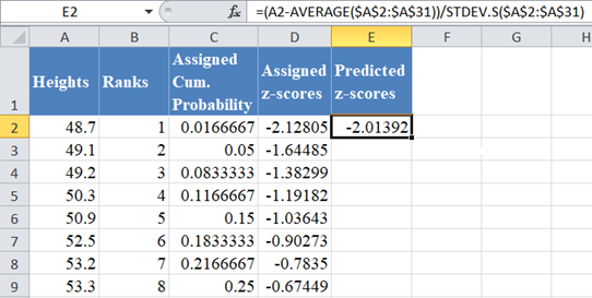
Complete the rest of the predicted z-score values as shown below:

Finally, switch the positions of the ‘Predicted z-score’ and the ‘Assigned z-score’ columns and plot a scatter plot following the procedure shown in the P–P plot section with the ‘Predicted z-score’ column on the x-axis and the ‘Assigned z-score’ on the y-axis as shown below:

Then, add the trend line to the graph as described in the P–P plot section as shown below:

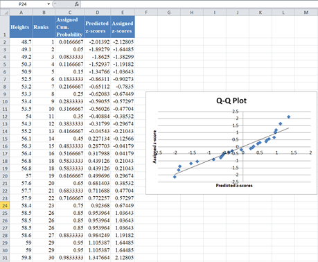
From the Q–Q plot, we can see that a lot of the data points digress significantly from the trend line, hence we can conclude that the data is not normally distributed.

Test for Normality in Google Sheets

Test for normality can be conducted in Google Sheets in a similar way as done in Excel.

Histogram in Google Sheets

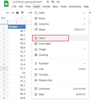
To construct a histogram in Google Sheets, highlight the dataset and click Insert > Chart as shown below:

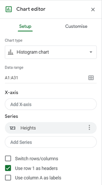
On the Chart Editor, in the Setup tab, set the Chart type to Histogram chart from the Other section, check the Use row 1 as headers checkbox if the title is included in your highlighted data range, and make other adjustments you may need. This is shown in the picture below:

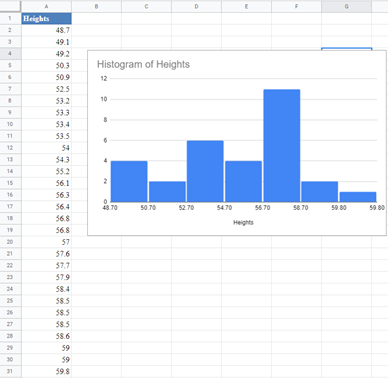
In the Customise tab, in the Histogram option, set the Bucket size to the desired interval width of the dataset. In our case, the interval width is 2 as shown in the picture below:

And we have the following output:

Boxplot in Google Sheets

Google Sheets does not have a boxplot template included in its chart templates. However, you can use the Candlestick chart to create a similar chart to a boxplot except that the median value is not included in a candlestick chart. Hence, you may not be able to adequately make a conclusion regarding the normality of a dataset using a candlestick chart.

P-P Plot and Q-Q Plot in Google Sheets

The P-P and the Q-Q plots can be constructed in Google Sheets in a similar way as it is constructed in Excel. To construct the P-P and the Q-Q plots in Google Sheets, use the same methods as explained in the P-P plot and the Q-Q plot sections for Excel above to obtain the axis to be used to construct the plot.

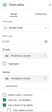
Next, highlight the Predicted Normal Cumulative Probability and the Assigned Cumulative Probability columns for the P-P plot or the Predicted z-score and the Assigned z-score columns for the Q-Q plot and click Insert > Chart.

On the Chart Editor, in the Setup tab, set the Chart type to Scatter chart. Google Sheets will usually plot the two columns as two independent plots, so to change this, select the correct x-axis column in the X-axis option and remove the x-axis column from the Series options. So, in our case, set the X-axis to “Predicted z-scores” for the Q-Q plot or the “Predicted Normal Cum. Probability” for the P-P plot. Then remove them from Series, by clicking three dots at their side and clicking Remove. The settings for the Q-Q plot are shown in the picture below:

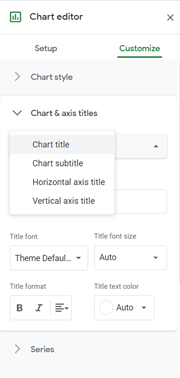
In the Customise tab, set the Chart title, the Horizontal axis title and the Vertical axis title in the Chart & axis titles option:

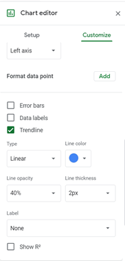
Check the Trendline checkbox in the Series option:

And we have the following output: