Reverse Text in Excel & Google Sheets
Written by
Reviewed by
Download the example workbook
This tutorial will demonstrate how to reverse text in a cell in Excel & Google Sheets.
Reverse Text – Simple Formula
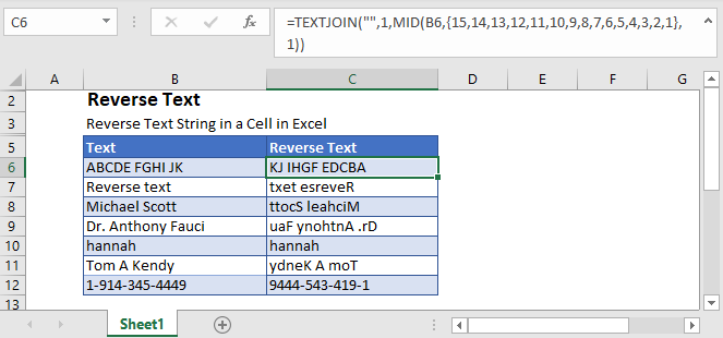
The simplest way to reverse a text string in Excel is with the TEXTJOIN and MID functions.
=TEXTJOIN("",1,MID(B6,{15,14,13,12,11,10,9,8,7,6,5,4,3,2,1},1))
Note: This formula will only work for text with 15 characters or less. To work with longer text strings, you must add a larger array constant or use the Dynamic Array formula below.
How Does this Formula Work?
The MID Function extracts character(s) from a string of text. In our example, we told the MID Function to only extract one character. Then by defining the array constant {15,14,13,12,11,10,9,8,7,6,5,4,3,2,1} as the start position, the MID Function will output the text in reverse order.
The TEXTJOIN Function joins the array constant result together, outputting the text in reverse order.
Reverse Text – Dynamic Array
The simple formula will only reverse the first fifteen characters. To reverse more characters you would need to add to the array constant, or you can use the dynamic formula shown below.
The dynamic formula consists of the TEXTJOIN, MID, ROW, INDIRECT, and LEN functions.
Step 1
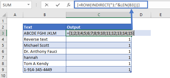
The first step is to calculate the total number of characters in the text string and generate an array of numbers corresponding to the number of characters:
=ROW(INDIRECT("1:"&LEN(B3)))
The above formula is an array formula and you can also convert the formula into array formula by pressing Ctrl + Shift + Enter. This is going to add curly brackets {} around the formula (note: this is not necessary in versions of Excel after Excel 2019).
Note: When these Formulas are entered in the cell, Excel will display only the first item in the array. To see the actual result of the array formula, you need to select the array formula cell and press F9 in the formula bar.
Step 2
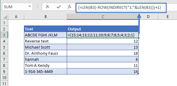
Next reverse the array of numbers that were generated in the previous step:
=LEN(B3)-ROW(INDIRECT("1:"&LEN(B3)))+1
Step 3
Now use the MID Function to extract the text.
This formula will reverse the order of the array during extraction by taking the characters from right to left.
=MID(B3,LEN(B3)-ROW(INDIRECT("1:"&LEN(B3)))+1,1)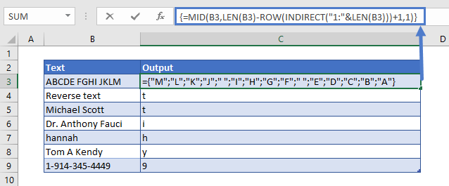
Final Step
Last use the TEXTJOIN Function to join together the individual characters.
=TEXTJOIN("",TRUE,MID(B3,LEN(B3)-ROW(INDIRECT("1:"&LEN(B3)))+1,1))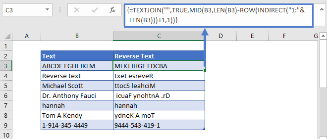
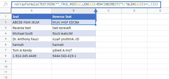
Reverse Text In Google Sheets
The formula to reverse text works exactly the same in Google Sheets as in Excel. Except when you close the formula with CTRL + SHIFT + ENTER, Google Sheets adds the ARRAYFORMULA function around the formula.
Reverse Text in VBA
To reverse a string of text using VBA, you can use the STRREVERSE Function:
Sub ReverseString()
Dim inputString As String
Dim reversedString As String
‘ Read Range A1 to a string variable
inputString = Range(“a1”).Value
‘ Reverse the string
reversedString = StrReverse(inputString)
‘ Output the result to range B1
Range(“b1”).Value = reversedString
End Sub
This Macro reverses the text found in range A1 and outputs the text to range B1. Follow the instructions here for directions for adding a macro to your workbook.

