Apply Conditional Formatting to Multiple Rows in Excel & Google Sheets
Written by
Reviewed by
In this article, you will learn how to apply conditional formatting to multiple rows in Excel and Google Sheets.
Apply Conditional Formatting to Multiple Rows
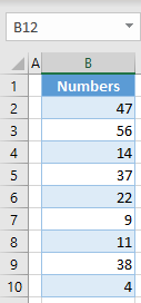
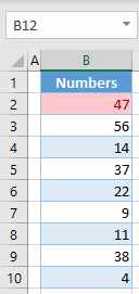
If you have conditional formatting in one cell in Excel, you can apply it to multiple rows in a few different ways. Let’s show first how to create a conditional formatting rule for one cell. Say you have the list of numbers below in Column B.
Create Conditional Formatting in a Single Cell
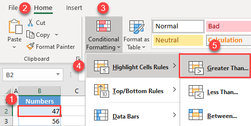
First, create a rule that highlights cell B2 in red if its value is greater than 20.
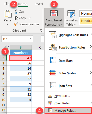
- Select a cell and in the Ribbon, go to Home > Conditional Formatting > Highlight Cells Rules > Greater Than.
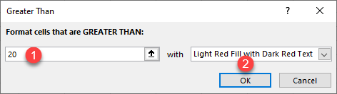
- In the pop-up window, enter 20 and click OK, leaving the default formatting (Light Red Fill with Dark Red Text).
Cell B2 is formatted in red, because its value is greater than 20.
Next, we’ll show how to apply this formatting to other rows in the range.
Apply to More Cells by Copy-Pasting
The first option is to use copy-paste to copy only formatting to other cells.
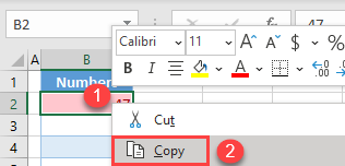
- Right-click a cell with conditional formatting and click Copy (or use the keyboard shortcut CTRL + C).
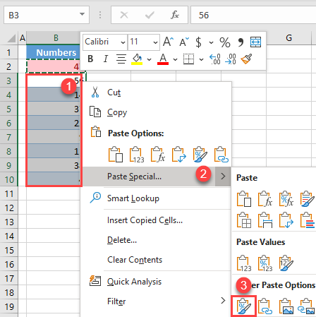
- Select and right-click a range where you want to paste the conditional formatting. Then click on the arrow next to Paste Special and choose Formatting.
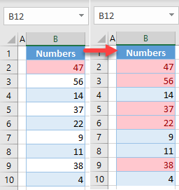
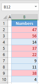
As a result, the formatting rule is copied to the whole range, and all cells with numbers greater than 20 are now red (B3, B5, B6, and B9).
Note: In this example, there’s a fixed value in the formatting rule. In cases where you have formulas as rules, you must pay attention to cell references in those formulas when copying the formatting.
Edit Conditional Formatting Rules
Instead of copying and pasting formats, you can edit the conditional formatting rules to extend the range they’re applied to. Each formatting rule has a range assigned to it. In this case, the range is cell B2. To edit a rule and apply conditional formatting for multiple rows, follow these steps:
- Select a cell with a conditional formatting rule and in the Ribbon, go to Home > Conditional Formatting > Manage Rules.
- In the Rules Manager window, (1) set the range to =$B$2:$B$10 in the Applies to box and (2) click OK.
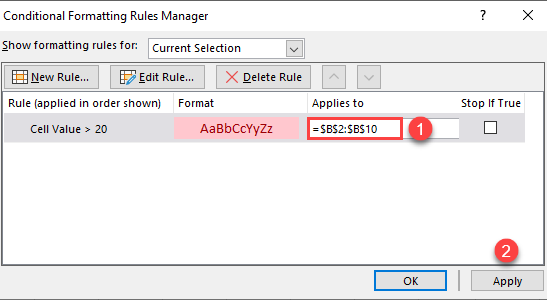
The output is exactly the same as in the previous section: All cells with numbers greater than 20 are highlighted.
Apply Conditional Formatting to Multiple Rows in Google Sheets
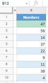
You can also apply conditional formatting to multiple rows in Google Sheets in the same ways shown above. Let’s first show how to create a conditional formatting rule for one cell.
Create Conditional Formatting in a Single Cell
To create a rule in cell B2 that will highlight the cell if the value is greater than 20, follow these steps:
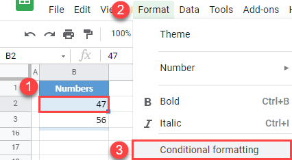
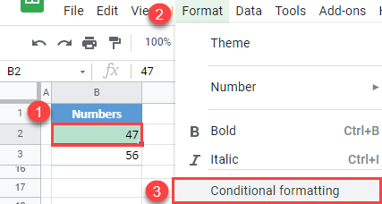
- Select the cell, and in the Menu, go to Format > Conditional formatting.
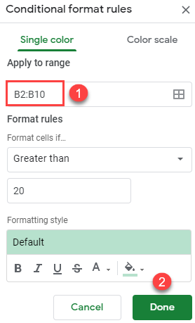
- In the formatting window on the right side, (1) select Greater than under Format rules, (2) enter 20, and (3) click Done.
This keeps the default formatting color (green), but you can change it if you want by clicking on the Fill color icon.
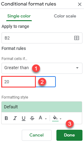
Since the value of cell B2 is 47, greater than 20, the cell is highlighted in green.
Apply to More Cells by Copy-Pasting
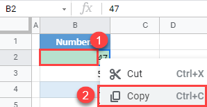
- Right-click a cell with a conditional formatting rule and click Copy (or use the keyboard shortcut CTRL + C).
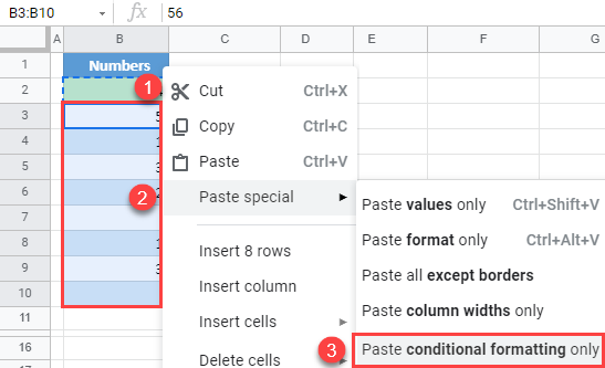
- Select and right-click the range where you want to paste the formatting rule (B3:B10), (2) click Paste special, and (3) choose Paste conditional formatting only.
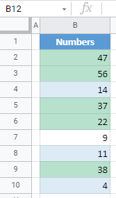
As a result, the formatting rule is applied to the entire data range in Column B (B2:B10).
Edit Conditional Formatting Rules
As in Excel, you can also edit the existing rule to expand the formatted range.
- Select a cell with conditional formatting (B2), and in the Menu, go to Format > Conditional formatting.
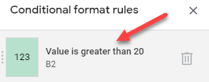
- On the right side of your browser, the conditional formatting window appears, showing the rules assigned to the selected cell. Click on the rule to edit it.
- Set the range to B2:B10 and click Done.
Again, the rule is now applied to the entire range.
