How To: Grade Formulas in Excel & Google Sheets
Written by
Reviewed by
Download the example workbook
This tutorial will demonstrate how to grade formulas in Excel and Google Sheets.
To grade a score achieved in an assignment, we can use the VLOOKUP or IF Functions.
VLOOKUP Function
The VLOOKUP Function searches for a value in the leftmost column of a table and then returns a value a specified number of columns to the right from the found value.
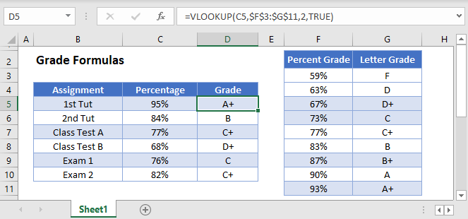
Firstly, we would need to have a table with the lookup values in it.
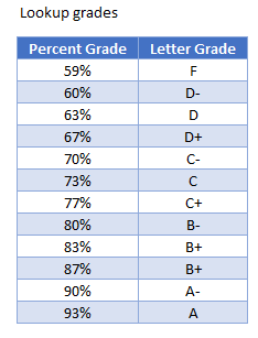
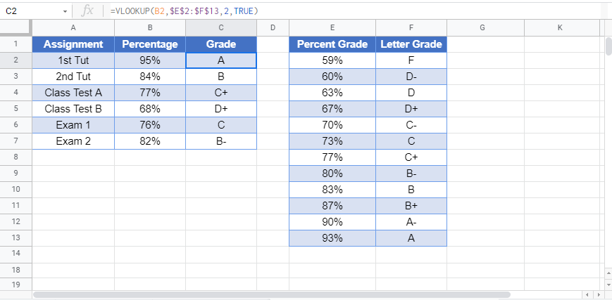
The Percentage obtained will be in the first column, while the corresponding Letter Grade will be in the second column. You will notice that the table is sorted from the lowest to the highest grade – this is important as you will see in the next section.
Next, we would type the VLOOKUP Formula where required. In the syntax of the VLOOKUP, after we specify the column to return form the look up, we are then given the opportunity to look for an EXACT match, or an APPROXIMATE match.

=VLOOKUP(C5,$F$5:$G$16,2,TRUE)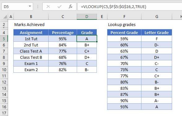
We are therefore going to look up the value in C5 from the range F5:G16 and return the value from the second column. Therefore, when the value is found in column F, the corresponding value in column G will be returned.
Notice that we have used the word TRUE in the last argument of the VLOOKUP – this means that an APPROXIMATE match will be obtained in the lookup. This enables the lookup to find the closest match to 95% contained in C5 – in this case, the 93% stored in F16.
When a VLOOKUP uses the TRUE argument for the match, it starts looking up from the BOTTOM of the table, which is the reason it is so important to have the table sorted from smallest to largest to obtain the correct letter grade.
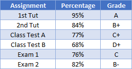
As we have used an absolute reference (F4 or the $ sign) for the table – $F$5:$G$16, we can copy this formula down from row 5 to row 10 to obtain the grades for each of the assignments.
IF Function
The IF Function will also work to get the correct letter Grade for the assignments; however, it will be a much longer formula as you will need to use multiple nested IF statements to obtain the correct grade.
Firstly, we can use an IF Function to look up 4 simple grades – A, B, C and D.
=IF(C5>90%,"A", IF(C5>80%,"B", IF(C5>70%,"C", IF(C5>60%, "D", "F"))))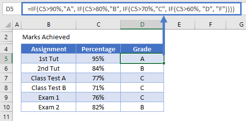
This formula contains 4 nested
statements and will grade the percentages based on the 4 letter grades provided.
If we want to break the grade down further, as with the VLOOKUP function, we can nest more IF statements into the formula where the IF statement can lookup the letter grade in a corresponding table.
=IF(C5>=$F$16,$G$16,IF(C5>=$F$15,$G$15,IF(C5>=$F$14,$G$14,IF(C5>=$F$13,$G$13,IF(C5>=$F$12,$G$9,IF(C5>=$F$11,$G$11,IF(C5>=$F$10,$G$10,IF(C5>=$F$9,$G$9,IF(C5>=$F$8,$G$8,IF(C5>=$F$7,$G$7,IF(C5>=$F$6,$G$6,$G$5)))))))))))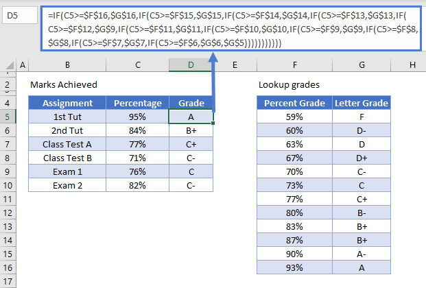
As with the lookup function, we can then copy the formula down to the rest of the rows.
Weighted Average
A weighted average is when assignments on a course differ in the credit value that they count towards the final course mark calculated. For example, during a year, a student may do tutorials, class tests and exams. The exams might count more towards the final mark for the course than the class tests of tutorials.
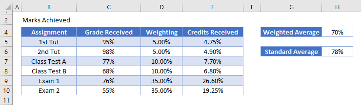
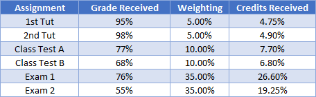
The weighting column in the example above adds up to the 100% total mark of the course. Each assignment has a weighting assigned to it. To work out the credits received for each assignment, we would need to multiply the percentage received by the weighting of the assignment.
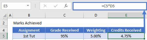
The credit received for the 1st Tut therefore is 4.75% of the 5% weighting available for that assignment. We can then copy that formula down to get the credits received for each of the assignments.
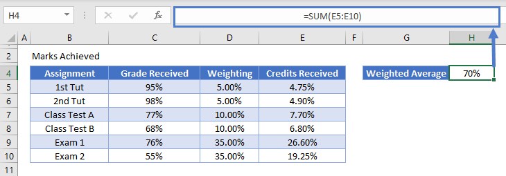
Once we have done this, we can sum up the credits received column to see the final course weighted average mark.
To see the difference between the weighted average, and the normal average, we can add up the grades received for all the assignments, and then divide these by the number of assignments.
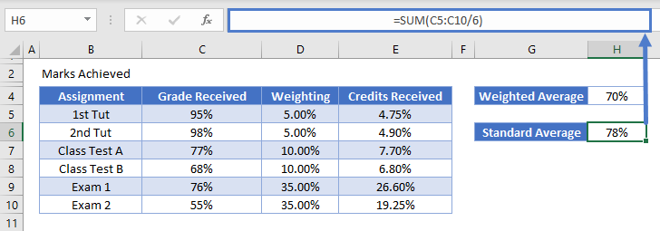
You will notice in the case of this student; the weighted average is lower than the standard average due to his poor performance in Exam 2!
How To Grade Formulas in Google Sheets
All the examples explained above work the same in Google sheets as they do in Excel.
LINK TO << vlookup-letter-grades>>

