Risk Score Bucket Using VLOOKUP – Excel & Google Sheets
Written by
Reviewed by
Download the example workbook
This tutorial will demonstrate how calculate a risk score bucket using VLOOKUP in Excel and Google Sheets.
A risk score matrix is a matrix that is used during risk assessment in order to calculate a risk value by inputting the likelihood and consequence of an event. We can create a simple risk score matrix in Excel by using the VLOOKUP and MATCH Functions.
Risk Matrix Excel
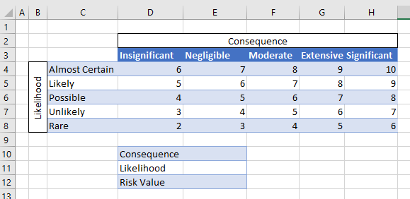
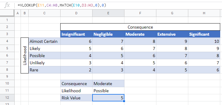
First, we would need to lay out the risk matrix as shown below.
Creating Drop Down Lists
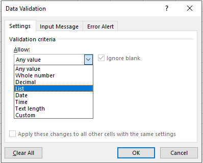
Next, we can use Data Validation to create drop down lists for the Consequence and Likelihood cells.
- Click in E10.
- In the Ribbon, select Data>Data Validation.
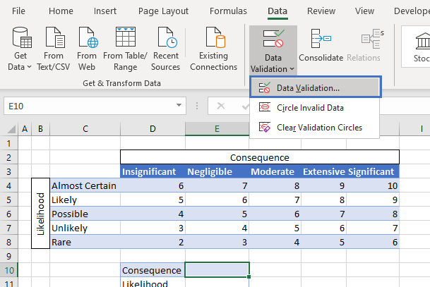
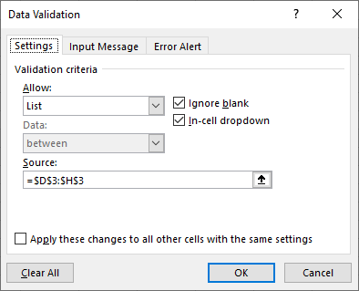
- Select List from the drop-down list provided.
- Highlight D3:H3 and then click OK.
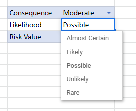
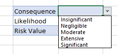
You will now have a dropdown list displaying the different categories for the Consequences of the Risk assessment.
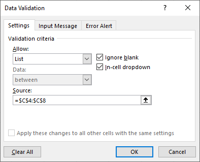
Repeat the data validation for the Likelihood list.
Calculate the Risk Score using VLOOKUP and MATCH
Once the Risk Matrix is setup, we can now use the VLOOKUP and MATCH Functions to lookup the Risk Factor from the matrix.
MATCH
First, we use the MATCH Function to find out which row we want the VLOOKUP Function to look for.
=MATCH(E10,C3:H3,0)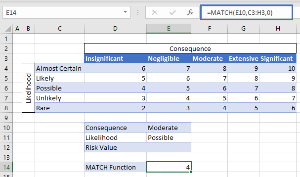
The MATCH Function above shows us that the Consequence ‘Moderate’ shown in E10 is in column 4 of the range C3:H3. This is therefore the column that the VLOOKUP Function will look in for the risk factor.
VLOOKUP
We now use the VLOOKUP Function to look up the Likelihood factor which is show as ‘Possible’ in E11.
=VLOOKUP(E11,C4:H8,E14,0)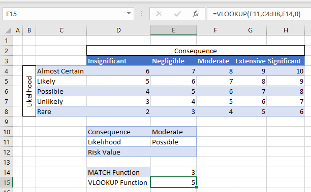
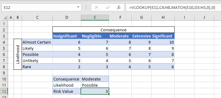
In the above example, the VLOOKUP is using the value in E14 as the column to look up. Joining the MATCH and VLOOKUP Functions will give us our original formula.
=VLOOKUP(E11,C4:H8,MATCH(E10,D3:H3,0),0)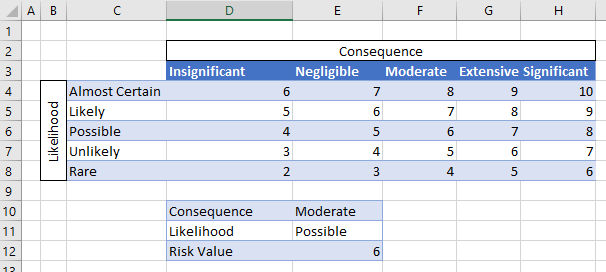
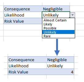
If you the Data Validation drop down lists to amend the Consequence and Likelihood criteria, the risk factor will change accordingly.
Risk Score Bucket Using VLOOKUP in Google Sheets
The Excel examples shown above work the same in Google Sheets as they do in Excel.
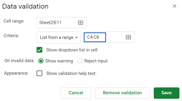
Data Validation in Google Sheets
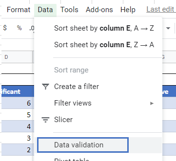
To create the dropdown list for the Consequence and Likelihood criteria, click in the cell where you want the list to go ex: E10.
From Menu bar, select Data >Data Validation.4
Select List from a range in the Criteria drop down box, and then select the range where the list is stored ex: D3:H3.
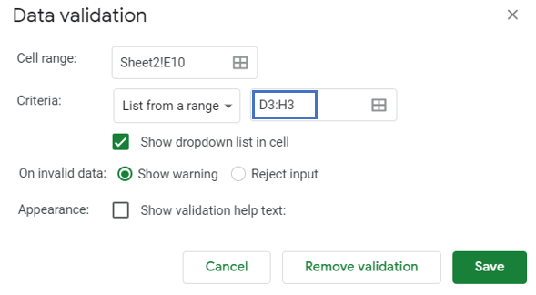
Click Save.
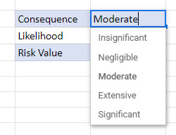
Your drop down list will be created.
Repeat the process for the Likelihood dropdown box.
Click Save.