SUBTOTAL IF Formula – Excel & Google Sheets

This tutorial will demonstrate how to calculate the “subtotal if”, performing the SUBTOTAL Function, only on cells that meet certain criteria.

SUBTOTAL Function

The SUBTOTAL Function is used to perform various calculations on a range of data (count, sum, average, etc.). If you’re not familiar with the function, you might be wondering why you wouldn’t just use the COUNT, SUM, or AVERAGE Functions themselves…  There are two good reasons:

1. You could create a table that lists the SUBTOTAL Options (1,2,3,4, etc.) and copy a single formula down to create summary data. (This could be an especially big time-saver if you’re attempting to calculate SUBTOTAL IF as we demonstrate in this article).
2. The SUBTOTAL Function can be used to calculate only visible (filtered) rows.

We will focus on the second implementation of the SUBTOTAL Function.

In this example, we will be using the function to count (COUNTA) visible rows by setting the SUBTOTAL function_num argument to 3 (A full list of possible functions can be found here.)

=SUBTOTAL(3,$D$2:$D$14)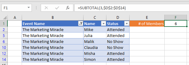

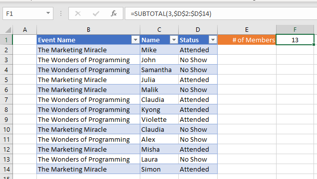
Notice how the results change as we manually filter rows.

SUBTOTAL IF

To create a “Subtotal If”, we will use a combination of SUMPRODUCT, SUBTOTAL, OFFSET, ROW, and MIN in an array formula. Using this combination, we can essentially create a generic “SUBTOTAL IF” function. Let’s walk through an example.

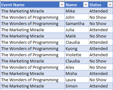
We have a list of members and their attendance status for each event:

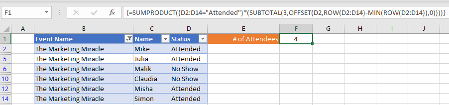
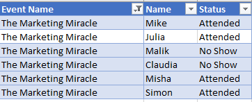
Supposed we are asked to count the number of members that have attended an event dynamically as we manually filter the list like so:

To accomplish this, we can use this formula:

=SUMPRODUCT((<values range>=<criteria>)*(SUBTOTAL(3,OFFSET(<first cell in range>,ROW(<values range>)-MIN(ROW(<values range>)),0))))

=SUMPRODUCT((D2:D14="Attended")*(SUBTOTAL(3,OFFSET(D2,ROW(D2:D14)-MIN(ROW(D2:D14)),0))))

When using Excel 2019 and earlier, you must enter the array formula by pressing CTRL + SHIFT + ENTER to tell Excel that you’re entering an array formula. You’ll know the formula was entered properly as an array formula when curly brackets appear around the formula (see image above).

How does the formula work?

The formula works by multiplying two arrays inside of SUMPRODUCT, where the first array deals with our criteria and the second array filters to visible rows only:

=SUMPRODUCT(<criteria array>*<visibility array>)

The Criteria Array

The criteria array evaluates each row in our values range (“Attended” Status in this example) and generates an array like this:

=(<values range>=<criteria>)

=(D2:D14="Attended")

Output:

{TRUE; FALSE; FALSE; TRUE; FALSE; TURE; TURE; TURE; FALSE; FALSE; TRUE; FALSE; TRUE}

Note that the output in the first array in our formula ignore whether the row is visible or not, which is where our second array comes in to help.

The Visibility Array

Using SUBTOTAL to exclude non-visible rows in our range, we can generate our visibility array. However, SUBTOTAL alone will return a single value, while SUMPRODUCT is expecting an array of values. To work around this, we use OFFSET to pass one row at a time. This technique requires feeding OFFSET an array that contains one number at time. The second array looks like this:

=SUBTOTAL(3,OFFSET(<first cell in range>,ROW(<values range>)-MIN(ROW(<values range>)),0))

=SUBTOTAL(3,OFFSET(D2,ROW(D2:D14)-MIN(ROW(D2:D14)),0))

Output:

{1;1;0;0;1;1}

Stitching the two together:

=SUMPRODUCT({TRUE; TRUE; FALSE; FALSE; TRUE; TRUE} * {1; 1; 0; 0; 1; 1})

= 4

SUBTOTAL IF with Multiple Criteria

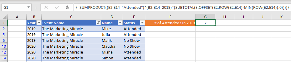
To add multiple criteria, simply multiple more criteria together within the SUMPRODUCT like so:

=SUMPRODUCT((<values range 1>=<criteria 1>)*(<values range 2>=<criteria 2>)*(SUBTOTAL(3,OFFSET(<first cell in range>,ROW(<values range>)-MIN(ROW(<values range>)),0))))

=SUMPRODUCT((E2:E14="Attended")*(B2:B14=2019)*(SUBTOTAL(3,OFFSET(E2,ROW(E2:E14)-MIN(ROW(E2:E14)),0))))

 

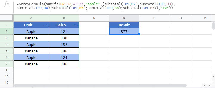
SUBTOTAL IF in Google Sheets

The SUBTOTAL IF Function works exactly the same in Google Sheets as in Excel. Except that notice when you use CTRL + SHIFT + ENTER to enter the array formula, Google Sheets adds the function ARRAYFORMULA to the formula (you can also manually add this function).