Sum & Sum If with VLOOKUP-Excel & Google Sheets
Written by
Reviewed by
Download the example workbook
This tutorial will demonstrate how to use the VLOOKUP Function nested in the SUMIFS Function to sum data rows matching a decoded value in Excel and Google Sheets.
VLOOKUP Within SUMIFS
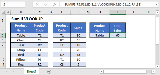
This example will sum the Total Sales for all Product Codes that match a given Product Name, defined in a separate reference table.
=SUMIFS(F3:F9,E3:E9,VLOOKUP(H3,B3:C9,2,FALSE))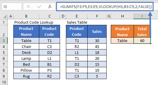
In this example, it is not possible to use the Product Name directly in the SUMIFS Function as the Sales Table only contains Product Codes. We need to convert the Name to a Code to calculate the Total Sales correctly.
Lets break down the formula into steps.
SUMIFS Function
If we know the Product Code (“T1”), then we can simply use the SUMIFS Function:
=SUMIFS(F3:F9,E3:E9,"T1")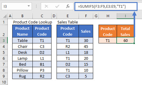
This formula sums all Sales corresponding to the Code “T1”.
VLOOKUP Function
However, if the Product Code does not provide enough information to make the summary useful, we need to allow a Product Name to be used instead. We can use the VLOOKUP Function to change the Name (“Table”) into its Code:
=VLOOKUP("Table",B3:C9,2,FALSE)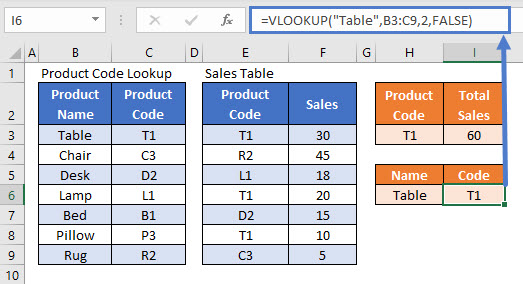
This formula finds “Table” in the Product Code Lookup data range and matches it to the value in the second column of that range (“T1”). We use FALSE in the VLOOKUP Function to indicate that we are looking for an exact match.
Using VLOOKUP Within SUMIFS – Cell References
Now that we’ve shown how to sum Sales by Code and how to look up Code by Name, we combine those steps into a single formula.
First, replace “Table” in the VLOOKUP Function with its cell reference (H3).
VLOOKUP(H3,B3:C9,2,FALSE)The input of the VLOOKUP is “Table”, and the output is “T1”, so we can replace “T1” in the SUMIFS Function with the VLOOKUP Function to get our final formula:
=SUMIFS(F3:F9,E3:E9,VLOOKUP(H3,B3:C9,2,FALSE))
Locking Cell References
To make our formulas easier to read, we’ve shown the formulas without locked cell references:
=SUMIFS(F3:F9,E3:E9,VLOOKUP(H3,B3:C9,2,FALSE))But these formulas will not work properly when copy and pasted elsewhere in your file. Instead, you should use locked cell references like this:
=SUMIFS($F$3:$F$9,$E$3:$E$9,VLOOKUP(H3,$B$3:$C$9,2,FALSE))Read our article on Locking Cell References to learn more.
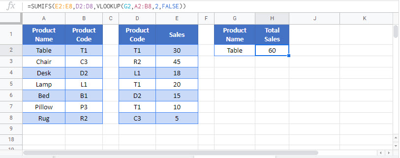
Sum if Using VLOOKUP in Google Sheets
These formulas work exactly the same in Google Sheets as in Excel.