SUBTOTAL Function Examples In Excel, VBA, & Google Sheets

This tutorial demonstrates how to use the SUBTOTAL Function in Excel to calculate summary statistics.

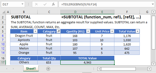
What is the SUBTOTAL function?

The SUBTOTAL Function Calculates a summary statistic for a series of data. Available statistics include ,but are not limited to average, standard deviation, count, min, and max.

The SUBTOTAL is one of the unique functions within spreadsheets because it can tell the difference between hidden cells and non-hidden cells. This can prove to be quite helpful when dealing with filtered ranges or when you need to setup calculations based on different user selections. Since it also knows to ignore other SUBTOTAL functions from its calculations, we can also use it within large summarized data without fear of double-counting.

Basic Summary with SUBTOTAL

Let’s say that you had a table of sorted product sales, and wanted to create totals for each product, as well as create an overall total. You could use a PivotTable, or you can insert some formulas. Consider this layout:

I’ve placed some SUBTOTAL functions in cells B5 and B8 that look like

=SUBTOTAL(9, B2:B4)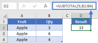

From the syntax, you can use a variety of numbers for the first argument. In our specific case, we’re using 9 to indicate we want to do a sum.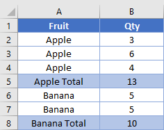

Let’s focus on cell B9. It has this formula, which includes the entire column B data range, but doesn’t include the other subtotals.

=SUBTOTAL(9, B2:B8)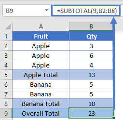

NOTE: If you don’t want to write all the summary formulas yourself, you can go to the Data ribbon and use the Outline – Subtotal wizard. It will automatically insert rows and place the formulas for you.

SUBTOTAL Hidden Rows

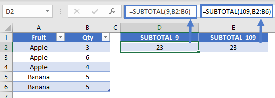
In the first example, we used a 9 to indicate we wanted to sum. Instead we can use 109 to sum. What’s the difference?

If you use the 1XX designations, the function will not include rows that have been manually hidden or filtered.

Here’s our table from before. We’ve shifted the functions over so we can see difference between the 9 and 109 arguments. With all visible, the results are the same.

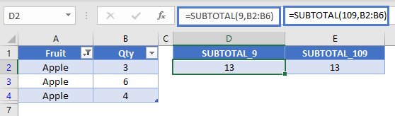
If we apply a filter to filter out the value of “Banana” in col A, the two functions remain the same.

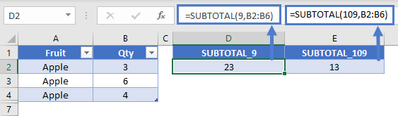
If we manually hide the rows, we see the difference. The 109 function was able to ignore the hidden row while the 9 function didn’t.

Change Math Operation with SUBTOTAL

You might like to sometimes be able to give your user the ability to change what type of calculations is performed. For instance, do they want to get the sum or the average. Since SUBTOTAL controls the math operation by an argument number, you can write this in a single formula. Here’s our setup:

We’ve created a dropdown in D2 where the user can select either “Sum” or “Average”. The formula in E2 is:

=SUBTOTAL(IF(D2="Average",1,IF(D2="Sum",9)),B2:B4)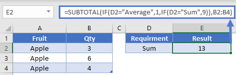

Here, the IF function is going to determine which numerical argument to give to the SUBTOTAL. If A5 is “Average”, then it will output a 1 and SUBTOTAL will give the average of B2:B4. Or, if A5 equals “Sum”, then the IF outputs a 9, and we get a different result.

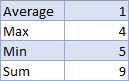
You could expand this capability by using a lookup table to list out even more types of operations you want to perform. Your lookup table might look like this

Then, you could change the formula in E2 to be

=SUBTOTAL(VLOOKUP(A5, LookupTable, 2, 0), B2:B4)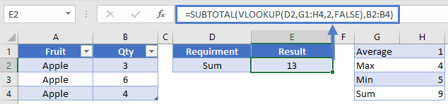

Conditional Formulas with SUBTOTAL

While SUBTOTAL has many operations it can do, it can’t check criteria on its own. However, we can use it in a helper column to perform this operation. When you have a column of data that you know will always have a piece of data in it, you can use SUBTOTALs ability to detect hidden rows.

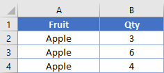
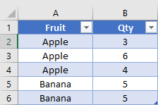
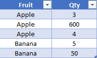
Here’s the table we’ll work with in this example. Eventually, we’d like to be able to sum the values for “Apple”, but also let the user filter the Qty column.

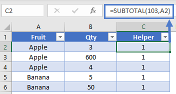
First, create a helper column which will house the SUBTOTAL function. In C2, the formula is:

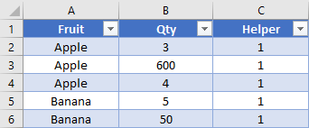
=SUBTOTAL(103, A2)

Remember that 103 means we want to do a COUNTA. I recommend using COUNTA because you can then have your reference cell of A2 be filled with either numbers or text. You’ll now have a table that looks like this:

This doesn’t appear helpful at first because all the values are just 1. However, if we hide row 3, that “1” in C3 will change to a 0 because it’s pointing at a hidden row. While it’s impossible to have an image showing the specific hidden cell’s value, you could check it by hiding the row and then writing a basic formula like this to check.

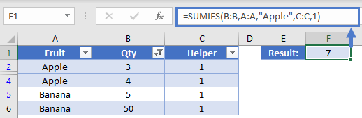
=C3

Now that we have a column that will change in value depending on if it’s hidden or not, we’re ready to write the final equation. Our SUMIFS will look like this

In this formula, we’re only going to sum values from column B when column A equals “Apple”, and the value in column C is 1 (aka, the row isn’t hidden). Let’s say that our user wants to filter out the 600, because it seems abnormally high. We can see that our formula gives correct result.

With this ability, you could apply a check to a COUNTIFS, SUMIFS, or even a SUMPRODUCT. You add in the ability to let your users control some table slicers, and you’re ready to create an awesome dashboard.

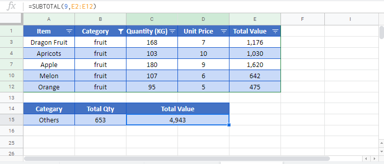
SUBTOTAL in Google Sheets

The SUBTOTAL Function works exactly the same in Google Sheets as in Excel:

SUBTOTAL Examples in VBA

You can also use the SUBTOTAL function in VBA. Type:

application.worksheetfunction.subtotal(function_num,reh1)

Executing the following VBA statements

Range("C7") = Application.WorksheetFunction.Subtotal(1, Range("C2:C5"))
Range("C8") = Application.WorksheetFunction.Subtotal(2, Range("C2:C5"))
Range("C9") = Application.WorksheetFunction.Subtotal(4, Range("C2:C5"))
Range("C10") = Application.WorksheetFunction.Subtotal(5, Range("C2:C5"))
Range("C11") = Application.WorksheetFunction.Subtotal(9, Range("C2:CE5"))

Range("D7") = Application.WorksheetFunction.Subtotal(1, Range("D2:D5"))
Range("D8") = Application.WorksheetFunction.Subtotal(2, Range("D2:D5"))
Range("D9") = Application.WorksheetFunction.Subtotal(4, Range("D2:D5"))
Range("D10") = Application.WorksheetFunction.Subtotal(5, Range("D2:D5"))
Range("D11") = Application.WorksheetFunction.Subtotal(9, Range("D2:D5"))

Range("E7") = Application.WorksheetFunction.Subtotal(1, Range("E2:E5"))
Range("E8") = Application.WorksheetFunction.Subtotal(2, Range("E2:E5"))
Range("E9") = Application.WorksheetFunction.Subtotal(4, Range("E2:E5"))
Range("E10") = Application.WorksheetFunction.Subtotal(5, Range("E2:E5"))
Range("E11") = Application.WorksheetFunction.Subtotal(9, Range("E2:E5"))

will produce the following results

 

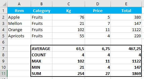
For the function arguments (function_num, etc.), you can either enter them directly into the function, or define variables to use instead.