Collapse Outline to Show Just Subtotals in Excel & Google Sheets
Written by
Reviewed by
This tutorial demonstrates how to collapse outline to show just subtotals in Excel and Google Sheets.
Collapse Outline to Show Just Subtotals
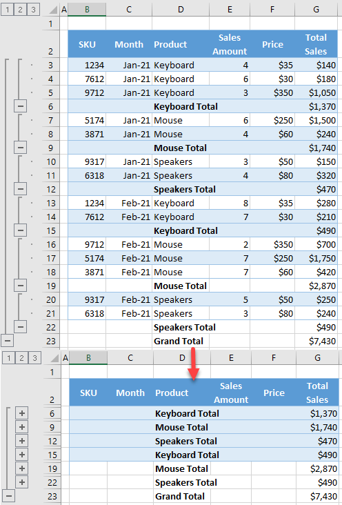
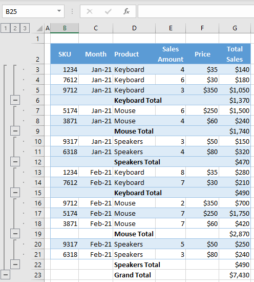
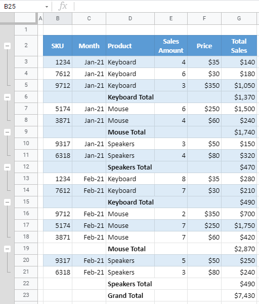
Say you have the following dataset with subtotals for every product in Column D.
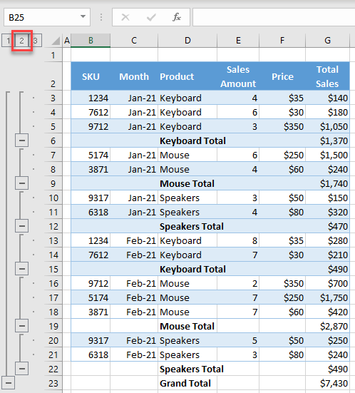
When you have the data grouped by a column and subtotals displayed, you can collapse detail levels, and display only subtotals. To achieve this, you need to click the outline bar number that you want to collapse (here, outline level 2).
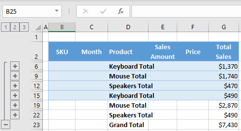
As a result, only subtotals for products are displayed, and detail lines are hidden.
In the outline bar, number 1 is always referring to the Grand Total, while subtotals get numbers starting from 2, as they are added. Suppose that you have two levels of subtotals and add a subtotal for months (Column C).
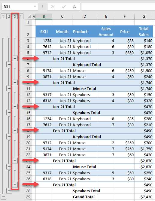
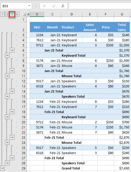
As you can see, now you have one more outline level (3) for month subtotals. To collapse these subtotals, you need to click number 3 in the outline bar.
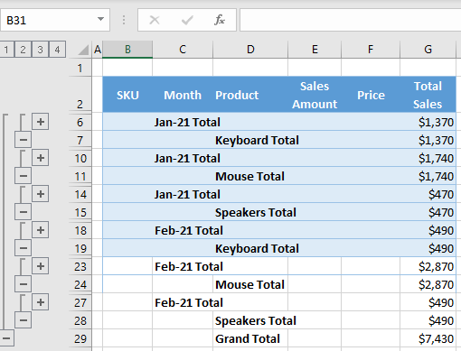
This collapses detail rows; only subtotals are displayed. This time, both month and product subtotals are displayed.
Collapse Outline to Show Just Subtotals in Google Sheets
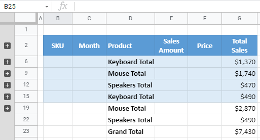
Let’s see how rows grouped by product look like in Google Sheets.
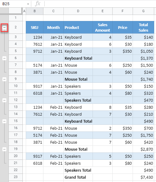
To collapse detail rows and display only subtotals per product, click the minus sign in the outline bar.
Now you have to repeat this step for every product group. In the end, only subtotal rows are displayed.