Create a Drop-Down List Filter in Excel & Google Sheets

This tutorial demonstrates how to create a drop-down list filter in Excel and Google Sheets.

 

 

You can use a drop-down list to extract rows of data that match the entry in the drop-down list, and return these rows to a separate area in the worksheet.

There are three main stages to complete this action.

1. Create a unique list of items to appear in the drop-down list as the data might contain repeating items.
2. Create the drop-down list to filter data.
3. Create the filter using helper columns that contain the formulas needed to extract the data.

Create a Unique List

For the first stage, you need a list of unique items for the field that will be filtered on (here, products).

1. Highlight the items that you want to appear in the drop-down list.

 

 

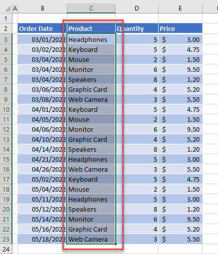
2. Then, copy and paste the list to a separate area of the worksheet.
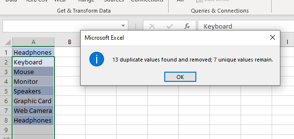
3. Remove the duplicates. Select the pasted list and then, in the Ribbon, go to Data > Data Tools > Remove Duplicates.

 

 

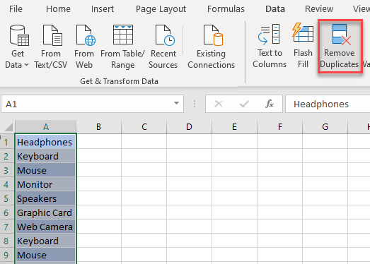
4. Click OK, and then click OK again to remove the duplicates and return to Excel. Now, there’s a unique list for the drop down.

 

 

Create the Drop-Down List

Now for the second stage, create the drop-down list for the filter.

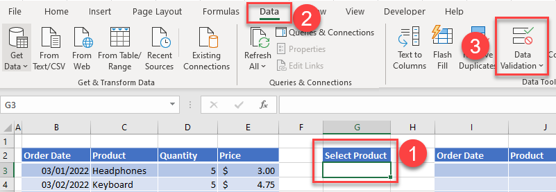
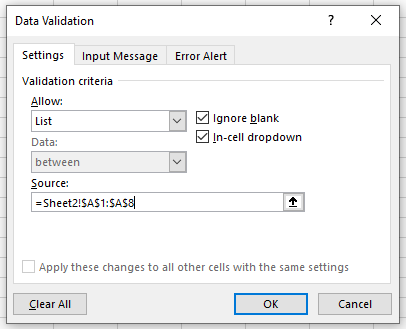
1. Select the cell where you wish to place the drop down, and then in the Ribbon, go to Data > Data Tools > Data Validation.

 

 

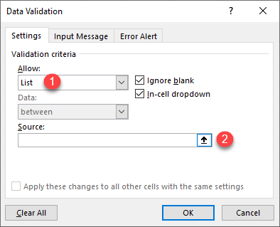
2. In the Data Validation window, choose List in the Allow drop down, and click on the arrow next to the Source box.

 

 

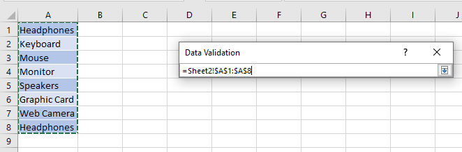
3. Select the range of cells that contain the unique items created above and press ENTER.

 

 

4. Click OK to confirm and exit the Data Validation window.

 

 

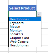
You can now select from the drop-down list.

 

 

Note: You can add your own error message for data validation. You can also add an input message to the cells with data validation in order to provide information on which values are allowed.

Extract Data With Formulas

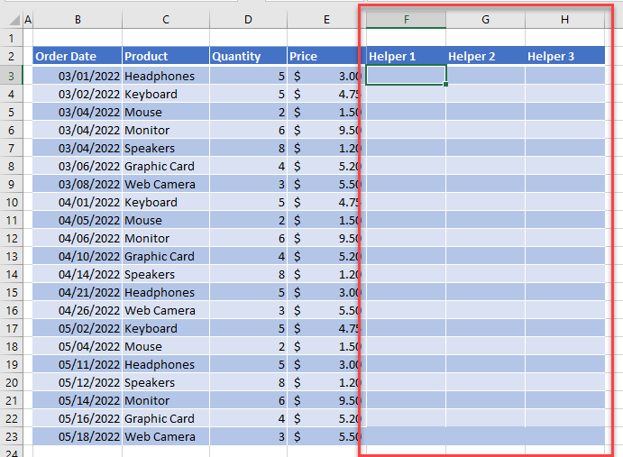
For the third and final stage, add columns of formulas that will act as filters alongside the drop-down list.

1. First, create “helper” columns in the table of data. To the right of the data table, insert three columns – Helper 1, Helper 2, and Helper 3.

 

 

2. Select the first cell in the Helper 1 column, and then type in the following ROWS formula:

=ROWS($B$3:B3)

Then, copy the formula down to the remaining rows in the helper column.

 

 

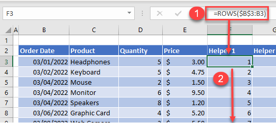
This formula gives each row in your data table a number, starting at the first row of data. Notice that it does not correspond with the row number in Excel.

3. Select the first cell in the Helper 2 column, and then type in the formula:

=IF(C3=$J$3,F3,"")

Copy the formula down to the remaining rows in the helper column.

 

 

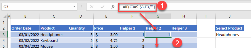
This formula returns the row number from the Helper 1 column if the value in the drop-down list (J3) is equal to the value in the same row in Column C (C3).

4. Now select the first cell in the Helper 3 column and type the following formula using the IFERROR and SMALL Functions:

=IFERROR(SMALL($G$3:$G$21,F3),"")

Then, copy the formula down to the remaining rows in the helper column.

 

 

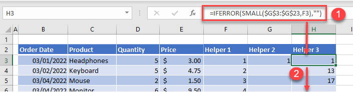
This formula returns the 1^st, 2^nd, 3^rd, etc. smallest number in the Helper 2 column based on the row number in the Helper 1 column.

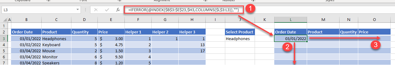
5. Now that you’ve created the helper columns, create the formula in the filter result table.
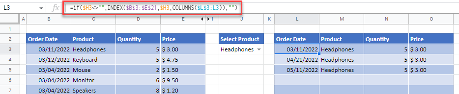
   Click in the first cell of the filter result table (e.g., L3), and then type in the following formula using the IFERROR, INDEX, and COLUMNS Functions:

=IFERROR(@INDEX($B$3:$E$21,$H3,COLUMNS($L$3:L3)),"")

Then, copy this formula down and across to fill up the remaining cells in the filter result table.

 

 

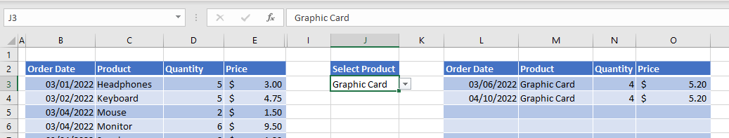
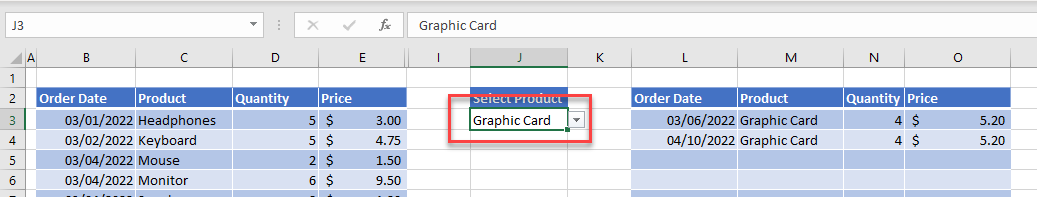
Depending on what value you have selected in the drop-down list, the filter results should show all the results for that value.
In this example, you have a list of product orders and you have filtered to show the orders where the product in the drop-down list selected is Headphones.

 

 

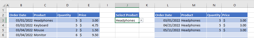
6. Change the selection in the drop-down list to show a different list of orders.

 

 

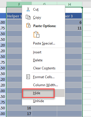
Note: To make the worksheet more aesthetically pleasing, and to protect the formulas in the helper columns, hide the helper columns. Right-click on the columns, then click Hide.

 

 

Create Drop-Down Filter in Google Sheets

The drop-down filter works the same in Google Sheets as it does in Excel. Follow the steps described above to create the drop-down list and three helper columns with the same formulas used for Excel.

When you create the final filter result table formulas, however, there is one slight difference:

=IF($H3<>"",INDEX($B$3:$E$21,$H3,COLUMNS($L$3:L3)),"")

Create an IF statement to check if the value in the Helper 3 column is there. If the value is there, you can run the INDEX formula, but if the value is not there, return a blank.