Insert a Picture Into a Cell Automatically in Excel & Google Sheets

This tutorial will demonstrate how to insert a picture into a cell automatically in Excel and Google Sheets.

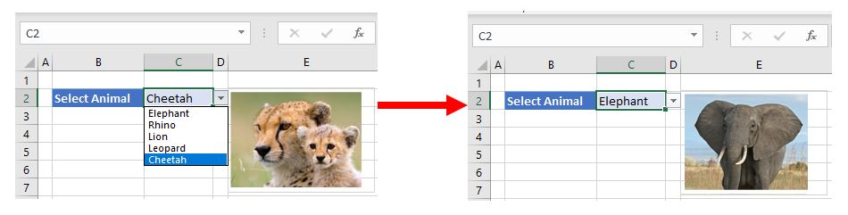
It’s possible to set it up a cell in Excel that shows an automatically changing picture depending on the user’s choice from a drop-down list. You can do this with a change event in VBA, but you can also follow the process below to avoid using macros.

Create Data List

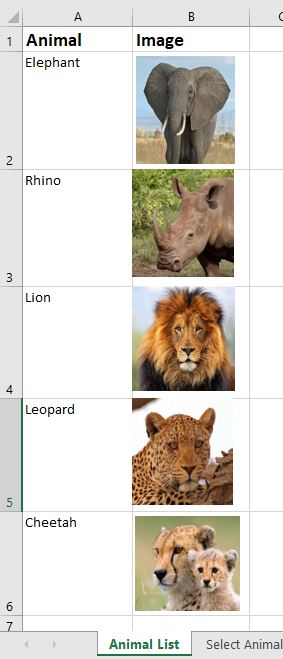
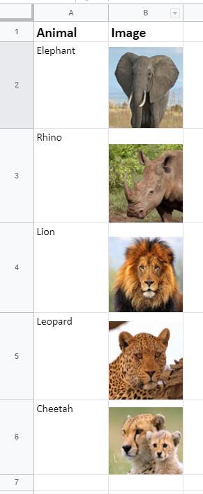
The first step in creating the example shown above is to create a list of animal names and images in a dedicated location in the workbook. It can be in a separate workbook from the drop-down list you’ll create, or a location in the same workbook.

Create Drop-Down List

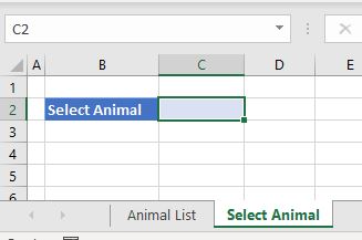
1. Next, select the cell where you want the drop-down list to go.

2. In the Ribbon, go to Data > Data Tools > Data Validation.

3. In the Settings tab, choose List under Allow, and check both Ignore blank and In-cell dropdown. Select the animal list range as the Source for the drop-down list.

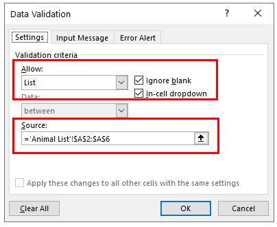
4. Click OK to add the data validation rule to the selected cell. This creates the first drop-down list showing the list of animals.

Create Range Name

The third step in creating a dynamic picture lookup is to create a range name.

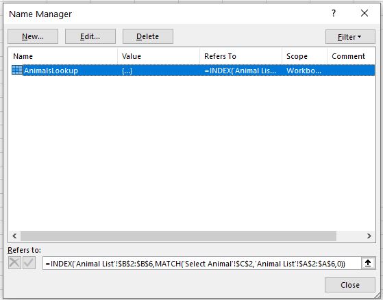
1. In the Ribbon, go to Formulas > Defined Names > Name Manager, then click New.

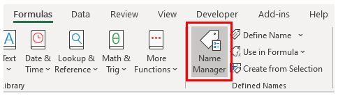
2. Call the Range name AnimalsLookup, then type the following formula in the Refers To box:

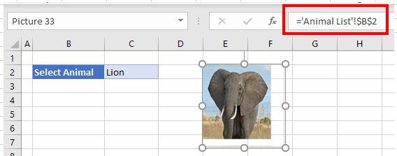
=INDEX('Animal List'!$B$2:$B$6,MATCH('Select Animal'!$C$2,'Animal List'!$A$2:$A$6,0))

• • The INDEX part of the formula must refer to the list of pictures that are in the animal list (e.g., B2:B6 in the Animal List sheet).
  • The MATCH part of the formula must match the cell where the drop-down list is located (e.g., C2 in the Select Animal sheet) to the list of animal names in the animal list (e.g., A2:A6 in the Animal List sheet).

3. Click OK to add the range name to the workbook.

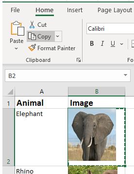
Create Linked Image

Now, link the image to the range name.

1. In the worksheet or location where the list of pictures is located, click the cell behind one of the animals and click Copy.

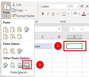
2. Select the cell where you want the picture to appear, next to the drop-down list. Then in the Ribbon, click Paste > Other Paste Options > Paste Linked Picture.

The image appears in the cell that has been selected. In the formula bar, you can see a formula linking the picture to the cell in the list of pictures, where it was originally copied from.

3. To link the formula to the named range, type in:

=ANIMALSLOOKUP

where AnimalsLookup is the range name for the list of animals and pictures in the Animals List sheet.

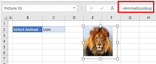
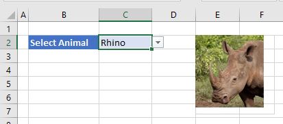
The picture automatically changes to whatever you choose from the drop-down list. Change the drop-down item to see a new picture appear!

Insert a Picture Automatically in Google Sheets

The process of linking a picture to a drop-down list is a lot easier in Google Sheets than it is in Excel. This is due to the fact that, unlike Excel, Google Sheets actually stores each image within the individual cell. This means you can simply do a lookup on the range where the names and pictures of the animals are stored.

1. As with Excel, first create a list of animals and insert pictures into the adjacent cells.
2. To insert an image into Google Sheets, position the cursor in the cell where you wish the image to go, and in the Menu, go to Insert > Image > Image in Cell.

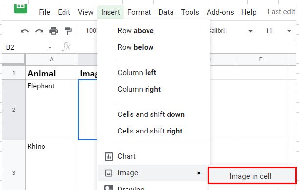
3. Browse to the URL of the image you need or upload it from a previously saved image. This inserts the image into the selected cell. Repeat the process to create a list of animal names and images.

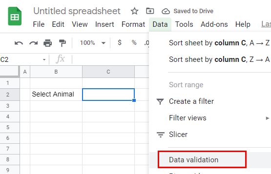
4. Next, select the cell where the drop-down list of animal names needs to appear, and in the Menu, go to Data validation.

5. Choose List from a Range as the Criteria, and then select the range where the animal names are stored e.g., ‘Animal List’! A2: A6.

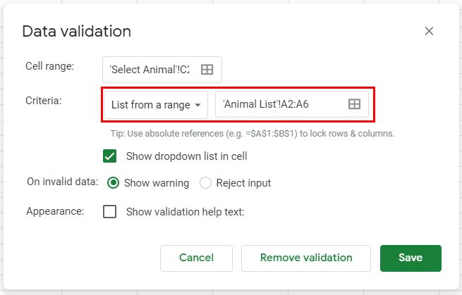
6. Click Save to save the drop-down list to the required cell (e.g., C2).

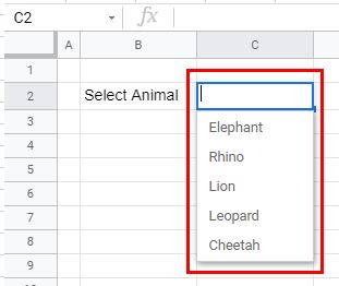
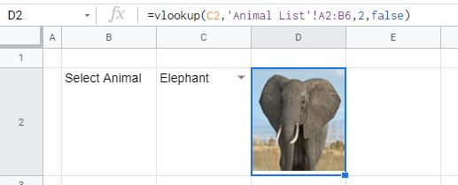
7. Select cell D2 and type in the VLOOKUP formula:

=VLOOKUP(C2,'Animal List'!A2:B6,2,false)

Select an animal from the list to show the corresponding animal image.

8. Change the size of the row to expand the image.