How to Get a Count via Pivot Table in Excel & Google Sheets
Written by
Reviewed by
This tutorial demonstrates how to count records from a dataset using a pivot table in Excel and Google Sheets.
Change the Pivot Table Value Field
Consider the pivot table below, based on a source dataset that has columns for each of the fields shown.
The Rows area has a field called Supplier in it, and the Values area has the sum of the Ordered field in it.
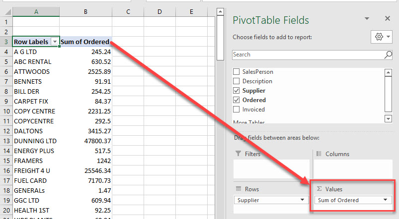
If you wish to count, rather than sum, the Ordered field, you need to change how the Values area is calculating.
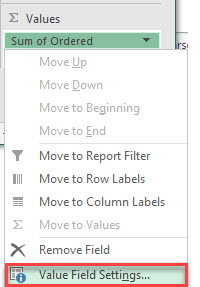
- Click the arrow to the right of Sum of Ordered, and then click Value Field Settings…
- Select Count from the Summarize value field by list. Optionally, you can set a new Custom Name; otherwise, the name defaults to the type of calculation (e.g., Count) and the original field name (e.g., Ordered).
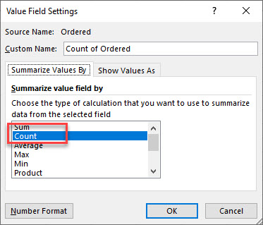
- Click OK to update the pivot table.
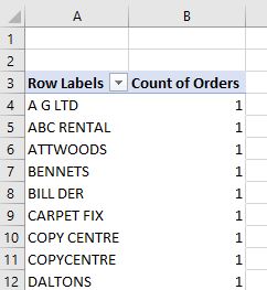
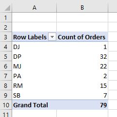
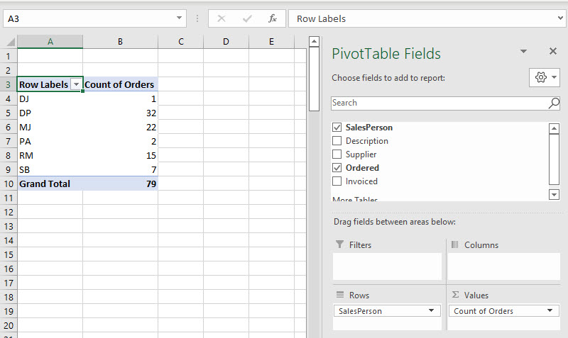
- If you switch the field in the Rows area from Supplier to Salesperson, the value field stays a count rather than a sum, and you can then see how many orders each salesperson made.
Tip: Try using some shortcuts when you’re working with pivot tables.
Pivot Table Count in Google Sheets
Consider the pivot table shown below.
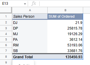
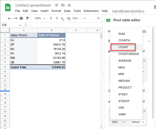
The Ordered field has been summarized using the SUM function in the Values section of the Pivot table editor.
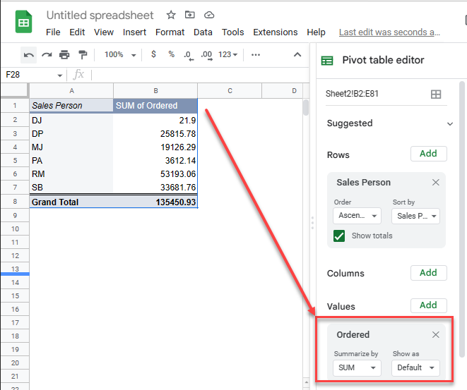
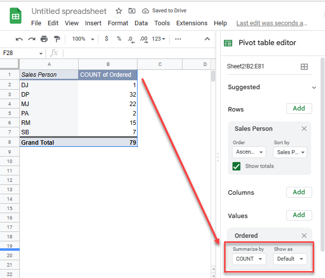
Just change SUM to COUNT in the Summarize by drop down.
The pivot table automatically updates to reflect how many orders each salesperson made rather than the added-up amount of the total orders.
See also: Count Unique Values With Pivot Table
