PERCENTILE IF Formula – Excel & Google Sheets
Written by
Reviewed by
Download the example workbook
This tutorial will demonstrate how to calculate “percentile if”, retrieving the kth percentile of only values that meet certain criteria.
PERCENTILE Function
The PERCENTILE Function is used to calculate the kth percentile of values in a range where k is the percentile value between 0 and 1 inclusive.
=PERCENTILE($D$2:$D$10,0.75)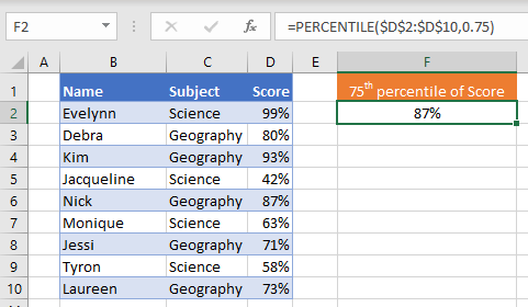
To create a “Percentile If”, we will use the PERCENTILE Function along with the IF Function in an array formula.
PERCENTILE IF
By combining PERCENTILE and IF in an array formula, we can essentially create a “PERCENTLE IF” function that works similar to how the built-in AVERAGEIF Function works.
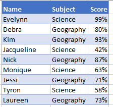
In this example, we have a list of scores achieved by students in two different subjects:
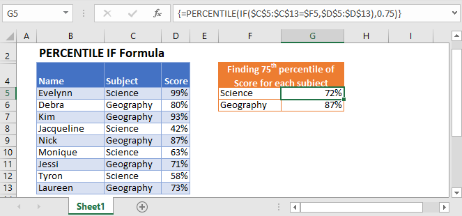
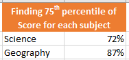
We want to find the 75th percentiles of scores achieved for each subject like so:
To accomplish this, we can nest an IF function with the subject as our criteria inside of the PERCENTILE function like so:
=PERCENTILE(IF(<criteria range>=<criteria>, <values range>),<percentile>)=PERCENTILE(IF($C$2:$C$10=$F3,$D$2:$D$10),0.75)When using Excel 2019 and earlier, you must enter the array formula by pressing CTRL + SHIFT + ENTER (instead of ENTER), telling Excel that the formula in an array formula. You’ll know it’s an array formula by the curly brackets that appear around the formula (see top image).
How does the formula work?
The If Function evaluates each cell in our criteria range as TRUE or FALSE, creating two arrays:
=PERCENTILE(IF({TRUE; FALSE;FALSE; TRUE; FALSE; TRUE; FALSE; TRUE; FALSE}, {0.99; 0.8; 0.93; 0.42; 0.87; 0.63; 0.71; 0.58; 0.73}), 0.75)Next, the IF Function creates a single array, replacing each value with FALSE if its condition is not met.
=PERCENTILE({0.81;FALSE;FALSE;0.42;FALSE;0.63;FALSE;0.58;FALSE}, 0.75)Now the PERCENTILE Function skips the FALSE values and calculates the 75th percentile of the remaining values (0.72 is the 75th percentile).
PERCENTILE IF with Multiple Criteria
To calculate PERCENTILE IF with multiple criteria (similar to how the built-in AVERAGEIFS function works), you can simply multiply the criteria together:
=PERCENTILE(IF((<criteria1 range>=<criteria1>)*(<criteria2 range>=<criteria2>),<values range>),<percentile>)=PERCENTILE(IF(($D$2:$D$10=$H2)*($C$2:$C$10=$G2),$E$2:$E$10),0.75)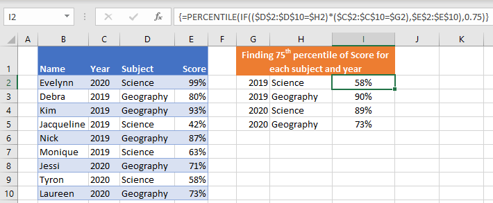
Another way to include multiple criteria is to nest more IF statements within the formula.
Tips and tricks:
- Where possible, always reference the position (k) from a helper cell and lock reference (F4) as this will make auto-filling formulas easier.
- If you are using Excel 2019 or newer, you may enter the formula without CTRL + SHIFT + ENTER.
- To retrieve the names of students that achieved the top marks, combine this with INDEX / MATCH.
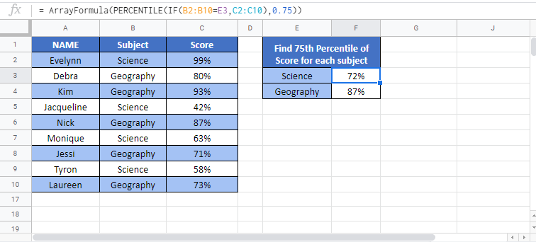
PERCENTILE IF in Google Sheets
The PERCENTILE IF formula works exactly the same in Google Sheets as in Excel, except that you must surround the formula with the ARRAYFORMULA Function to tell Google Sheets that it’s an array formula.