Apply Multiple Filters to Columns in Excel & Google Sheets

This tutorial demonstrates how to apply multiple filters to columns in Excel and Google Sheets.

 

 

► Click here to jump to the Google Sheets walkthrough.
► Click here for more on advanced filters.

Apply Multiple Filters to Columns

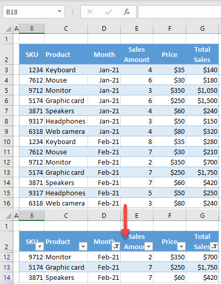
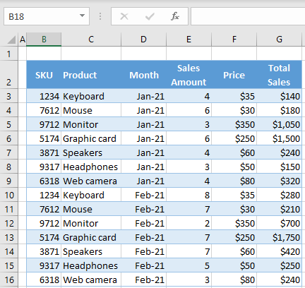
If you have a table with multiple columns in Excel, you can filter the data by multiple columns at once. Say you have the data table shown below.

 

 

To filter data first by month (display on Feb-21), and then by total sales (> $400), follow these steps:

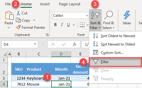
1. To display filter buttons in the column headings, select any cell in the data range (e.g., B2:G16), and in the Ribbon, go to Home > Sort & Filter > Filter.

 

 

Now every column heading has a filter button and can be used to filter the table data.

2. Click on the filter button for month (cell D2), check only February (uncheck January), and click OK. The filter functionality recognizes dates and groups them by year and month.

 

 

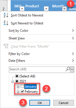
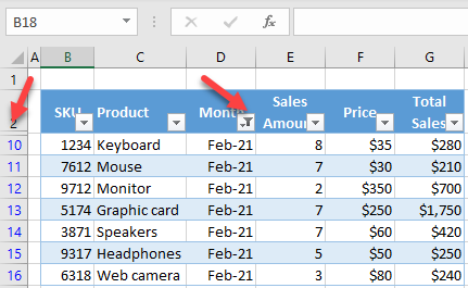
As a result of Step 2, all rows containing Jan-21 in Column D are filtered out, and only those with Feb-21 are displayed. Note that the appearance of the filter button for month (D2) is different, so it’s clear the range is filtered by month.

 

 

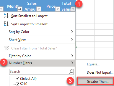
3. Now you can filter data by another column. Click on the filter button for total sales (G2), go to Number Filters > Greater Than…
   Note that you could also choose Equals, Does Not Equal, Less Than, etc.

 

 

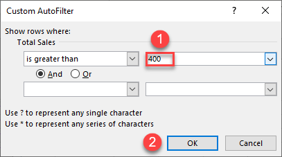
4. In the pop-up window, enter the lower limit (in this case, $400) and click OK. Here you could also add more conditions or change the operator.

 

 

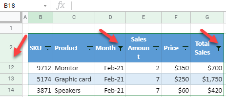
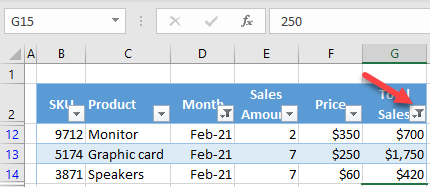
The final result is the original data range filtered by month (Feb-21) and by total sales (> $400).

 

 

Apply Multiple Filters in Google Sheets

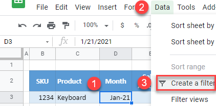
1. To create filter buttons, select any cell in the data range (B2:G16) and in the Menu, go to Data > Create a filter.

 

 

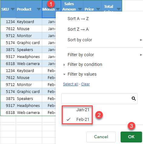
2. Click on the filter button for month (D2),choose only Feb-21 (uncheck Jan-21), and click OK.

 

 

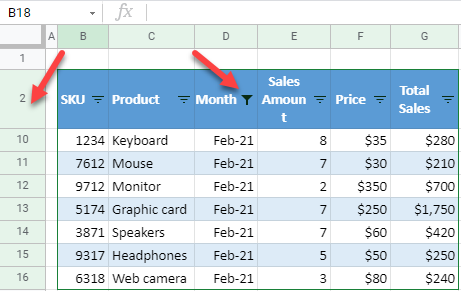
Now the data range is filtered by month, and only rows with Feb-21 are displayed while all other rows are hidden. Also, the filter button has a new appearance, so it’s clear there is an active filter on month.

 

 

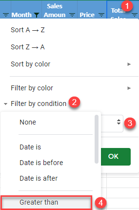
3. Click on the filter button for total sales (G2), go to Filter by condition > Greater than.
   As in Excel, you could alternatively choose Less than, Equal, etc.

 

 

4. In the text box that appears under the Greater than condition, enter a lower limit (400), and click OK.

 

 

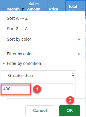
Finally, rows containing Feb-21 in Column D with a sales value greater than $400 are displayed, and other rows are hidden.