How to Flip a Table in Excel & Google Sheets

This tutorial demonstrates how to flip a table in Excel and Google Sheets.

Flip Rows and Columns in a Table

You can transpose data in Excel as long as the data is in a normal range and not in a table. If your data is formatted as a table, you must convert the data to a normal range before you can flip the table’s rows and columns.

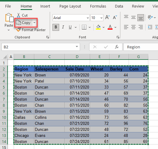
1. Once the table is formatted as a normal range, select the entire range.
2. Then, in the Ribbon, go to Home > Clipboard > Copy or press CTRL + C.

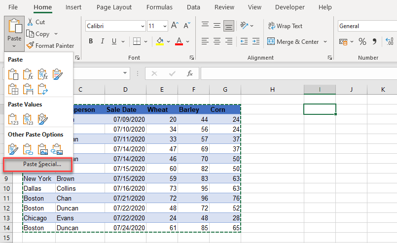
3. Click in the cell where you want to paste the flipped table, and then in the Ribbon, go to Home > Clipboard > Paste Special.

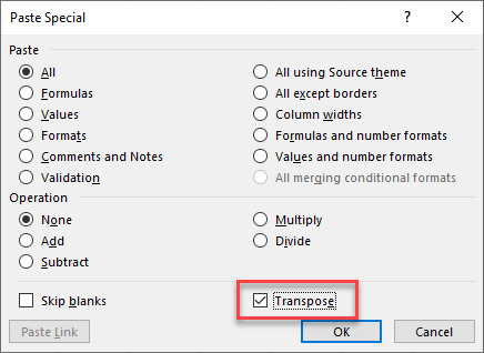
4. Tick the Transpose checkbox, and then click OK.

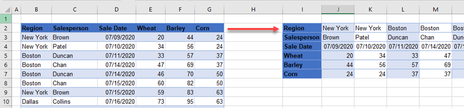
5. This flips the table, putting the row data in columns and the column data in rows.

Flip a Table Vertically

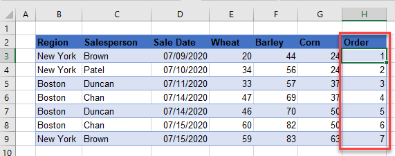
You can reverse the order of data in the rows of your table by using a “helper” column to determine the order of your data.

1. Add a helper column to the right side of your table filled with serial numbers starting from 1 and increasing by 1 in each row.

2. Click in the column, and then in the Ribbon, go to Home > Editing > Sort & Filter > Sort Largest to Smallest.

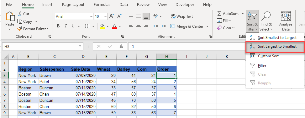
3. This sorts the rows in reverse order.

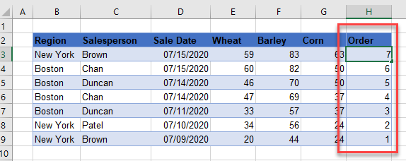
4. Delete the helper column (Order). Or, to keep a record of the original order, leave it in.

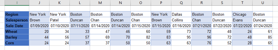
Flip a Table Horizontally

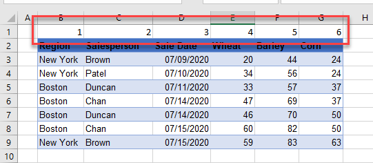
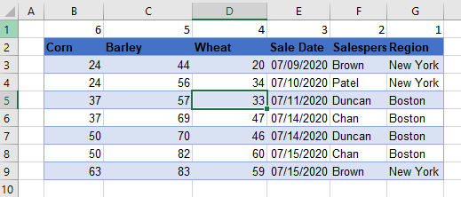
To switch the columns around, add a helper row and sort horizontally.

1. In the row directly above the table, add a helper row filled with serial numbers starting from 1 and increasing by 1 in each column.

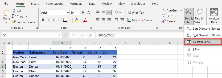
2. In the Ribbon, go to Home > Editing > Sort & Filter > Custom Sort.

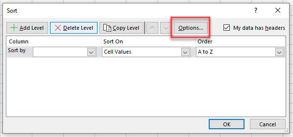
3. In the Sort dialog box, click Options…

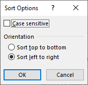
4. Choose Sort left to right as the Orientation, and then click OK.

5. In the Sort dialog box, choose to Sort by Row 1. Then, choose Cell Values in the Sort On drop down and Largest to Smallest in the Order drop down.

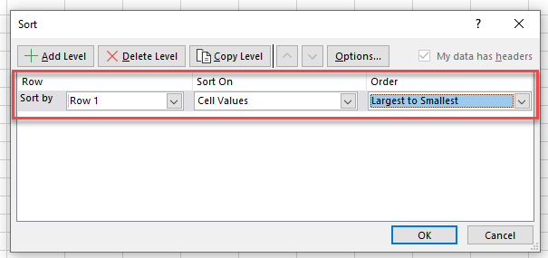
6. Click OK to sort. This reverses the column order.

Flip a Table in Google Sheets

You can flip your table in Google in the same way as you can do it in Excel.

Flip Rows and Columns

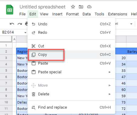
1. Select the dataset, and then in the Menu, go to Edit > Copy or press CTRL + C.

2. Select the cell where you want to paste your data, and then in the Menu, go to Edit > Paste Special > Transposed.

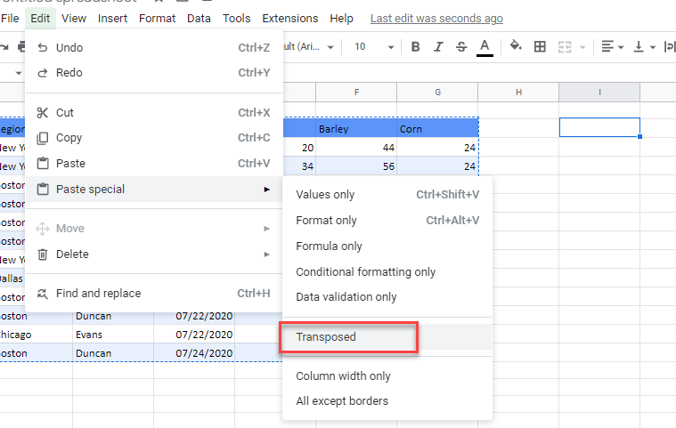
This pastes the dataset with the table information flipped.

Flip a Table Vertically

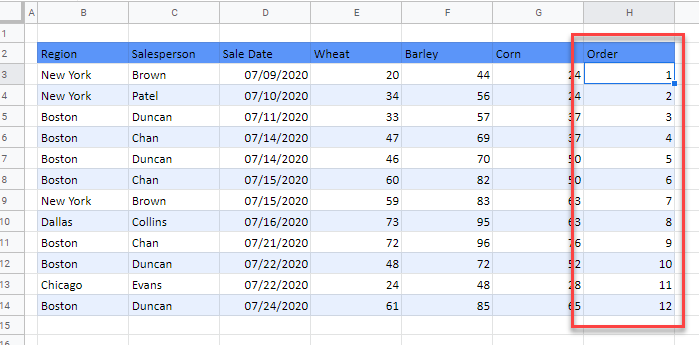
1. Add a helper column to your table. Fill with serial numbers starting from 1 and increasing by 1

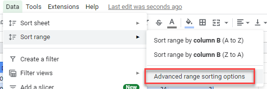
2. Highlight the entire table, and then in the Menu, go to Data > Sort range > Advanced range sorting options.

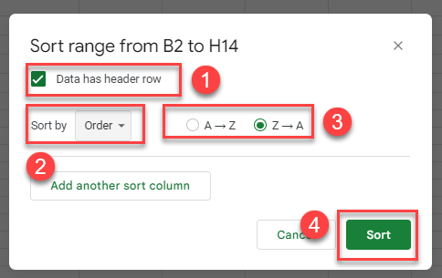
3. In the Sort range dialog box, tick Data has header row and then choose the column to sort by (Order). Then, choose to sort Z→A and click Sort.

As with Excel, your data is sorted in the reverse order compared to the original data.

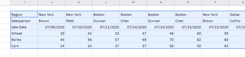
While Google Sheets does not have the same ability as Excel to flip a table horizontally, you can use the Transpose command to achieve a similar result.