Add a Calculated Field in a Pivot Table in Excel & Google Sheets

This tutorial demonstrates how to add a calculated field in a pivot table in Excel and Google Sheets.

 

 

Pivot tables make viewing and analyzing large amounts of data easy. For necessary calculations in your analysis, you can always add a column to your source data and include it as a pivot table field. But you can also calculate new fields right in the pivot table, without making any edits to your source data.

Tip: Try using some shortcuts when you’re working with pivot tables.

Add Pivot Table Calculated Field

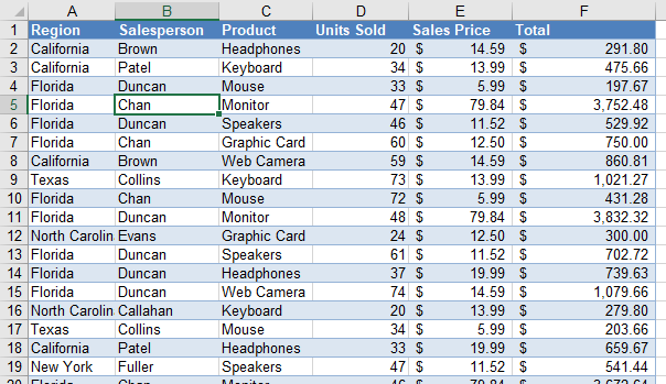
Say you have a pivot table created from the data table below.

 

 

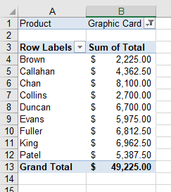
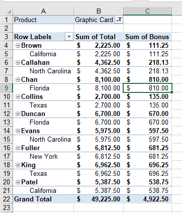
1. The pivot table is set up with the Product field as the filter, Salesperson as the rows, and the Total as the values.

 

 

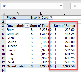
2. Now, add a calculated field that gives each salesperson a 10% bonus based on the total.
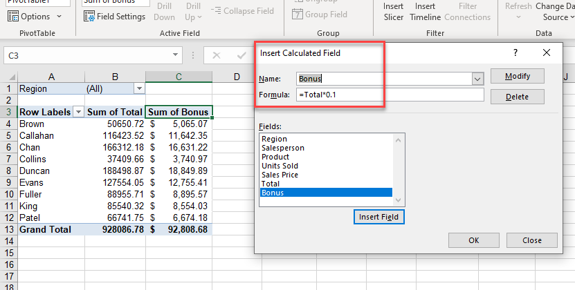
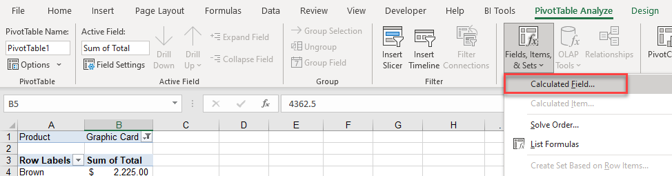
   In the Ribbon, go to PivotTable Analyze > Calculations > Fields, Items & Sets > Calculated Field…

 

 

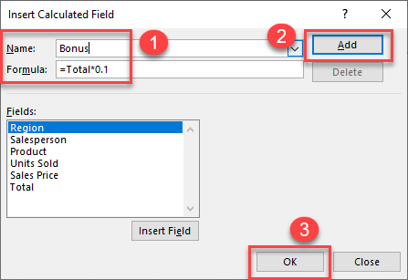
3. Type in a Name for the field, and then in the Formula box, type in your custom formula. Click Add to add your field to the Fields list below. Then, click OK to add the field to the pivot table.

 

 

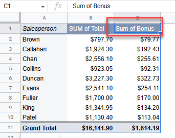
The additional field is added as the last column in this pivot table.

 

 

4. Your formula can be as simple or as complicated as necessary. For example, say you want to give a 10% bonus for sales over $5,000 but only a 5% bonus otherwise. Modify the Bonus formula to do this with an IF statement.

=IF(Total>5000,Total*0.1,Total*0.05)

5. In the Insert Calculated Field dialog box, choose the calculated field (here, Bonus) from the Name drop down, and then edit the formula accordingly.

 

 

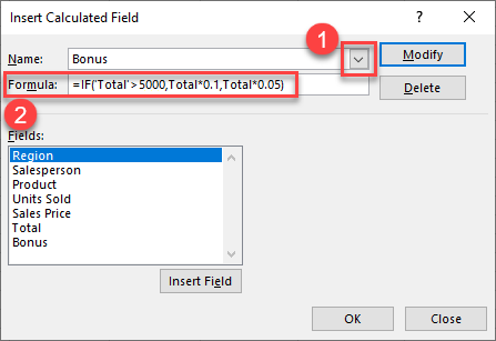
6. Click Modify and then OK to update your pivot table.

 

 

Calculated Pivot Table Field in Google Sheets

You can also add a calculated field as an additional column when you have a pivot table in Google Sheets.

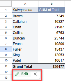
1. Click in your pivot table to show the pivot table editor pane on the right side of your screen. If the pane does not show, click the Edit button below your pivot table to make the pane visible.

 

 

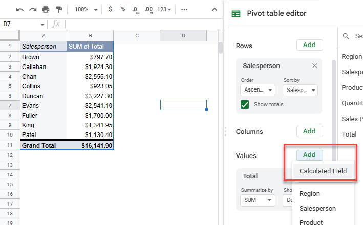
2. In the Pivot table editor, click the Add button in the values section, and then click Calculated Field.

 

 

3. Type the calculation in the Formula box. The pivot table updates automatically.

 

 

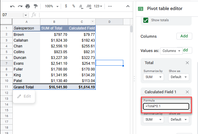
4. You can, optionally, rename the column for the calculated field. Just type the new name in the relevant cell in the pivot table.