Advanced Pivot Table Techniques in Excel and Google Sheets

This tutorial demonstrates advanced pivot table techniques in Excel and Google Sheets.

 

 

Click here for a briefer tutorial on creating a pivot table. Or read on to explore Excel’s more complex PivotTable features.

Pivot Table Source Data
Recommended Pivot Tables
Refresh Pivot Table Data
Group Pivot Table Fields
Pivot Table Filters
Create and Use Slicers With Pivot Tables
Format Pivot Table Values
Hide and Unhide Pivot Table Subtotals
Pivot Table Calculated Fields
Move Pivot Table
Insert Pivot Chart
Pivot Table Options
Google Sheets

Tip: Try using some shortcuts when you’re working with pivot tables.

What is “Source Data” in a Pivot Table?

The source data of a pivot table is the data that the pivot table is going to be created from. This has to be stored in the correct table structure or format to be able to create a successful pivot table. The data table has to consist of column (“field”) headers with logical names to explain the data below each column and rows of records.

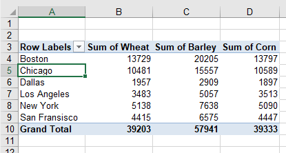
Consider the spreadsheet below:

 

 

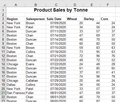
The data is set up in columns, each with a unique field name. Each row in Excel is known as a single record, and those records start directly below the header row. The data can’t contain any blank rows or columns. With the data set up correctly, you can create the pivot table. Choose from the Recommended PivotTables or design a new pivot table with the fields you need.

Recommended PivotTables

Excel has a feature to recommend a pivot table automatically based on your data.

1. Select any cell within your source data, and then in the Ribbon, go to Insert > Tables > Recommended Pivot Tables.

 

 

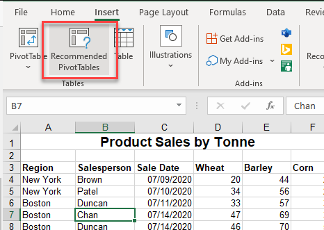
2. Choose a pivot table from the list on the left, and then click OK.

 

 

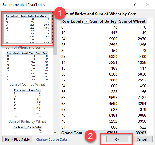
3. This creates a pivot table in a new sheet. You can then adjust it in the PivotTable Fields window. In the example above, Excel used the last column of data for row labels. This doesn’t make much sense! You can remove this field (Corn) from the row labels by dragging it across to the Values box.

 

 

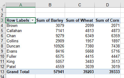
4. You can then drag a more appropriate field (Region, Salesperson, or Sale Date) to the Rows box.

 

 

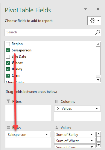
The pivot table changes accordingly.

 

 

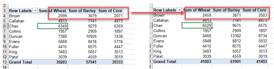
Refresh Pivot Table Data

If your source data changes, you need to refresh your pivot table; it won’t change automatically.

In the Ribbon, go to Data > Refresh All.

 

 

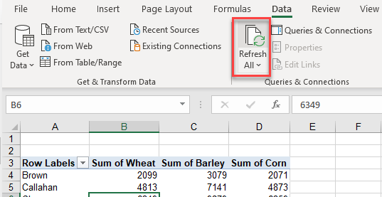
The figures in your pivot table now match the edited source data.

 

 

Group Pivot Table Fields

Group Row and Column Fields

You can group row and column fields if you have logical groups in your data.

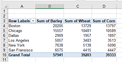
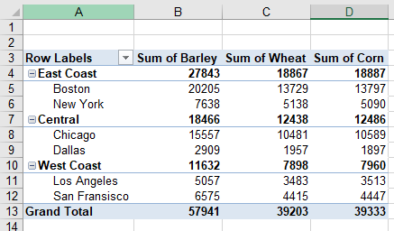
Consider the following pivot table.

 

 

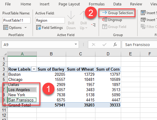
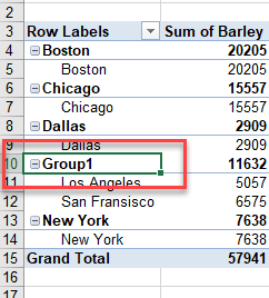
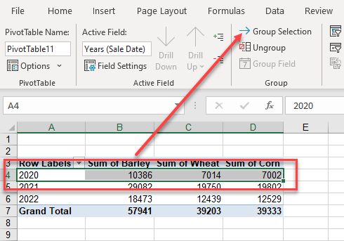
1. In the pivot table, hold down the CTRL key, and select the field values you wish to group. Then in the Ribbon, go to Pivot Table Analyze > Group > Group Selection.

 

 

2. The two row labels selected (here, Los Angeles and San Francisco) are grouped together under a new group called Group1.

 

 

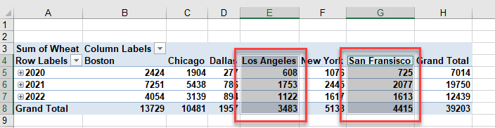
3. If your data is set up in a column format, you may wish to group by columns. Select the columns you wish to group on.

 

 

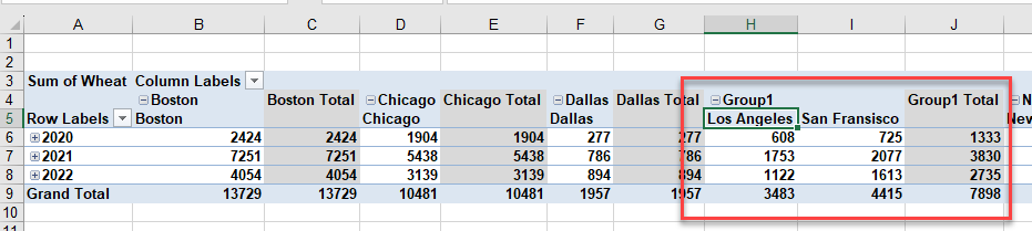
4. Then in the Ribbon, go to Pivot Table Analyze > Group > Group Selection.

 

 

Rename Groups

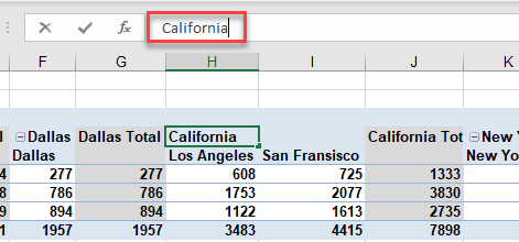
1. You can easily rename a group. Select the cell with the label, and in the formula bar, type in a new name for the group.

 

 

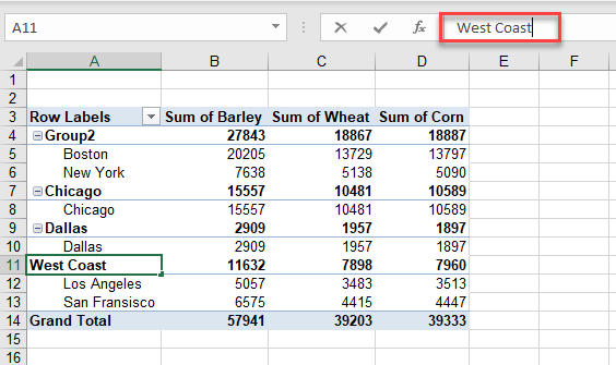
2. You can do this with each row group that’s created.

 

 

3. You can also rename your column groups.

 

 

Group by Date

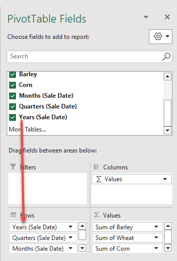
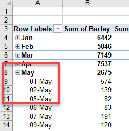
1. If you move the Sales Date to the Row Labels section of the pivot table, notice that the pivot table automatically groups the Sales Date by Year, Quarter, and Month. The actual dates of the order are below each month for that quarter and year.

 

 

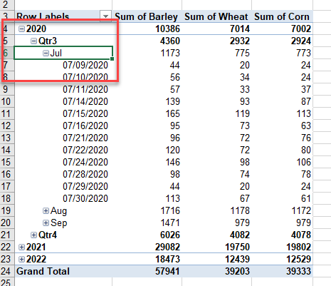
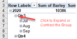
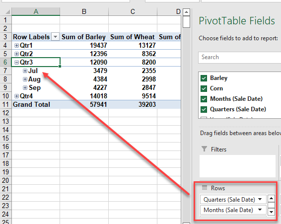
2. Each group has an expand (+) icon attached to it. If you click this icon, as shown in the graphic above, it changes to a collapse (–) icon.

 

 

3. The Rows area of PivotTable Fields reflects that as well as the Order Date (with automatic Quarters and Years) field have been created and added to the pivot table.

 

 

4. You can remove any of the automatically generated date fields (years, quarters, or months), but if you remove the year, for example, then the other date fields aggregate the yearly data. In other words, all the orders for February are included in Quarter1 > February (i.e., the sum of Feb 2020, Feb 2021, and Feb 2022).
   Similarly, if you remove the Quarters field, then only months are shown – so all the orders in February, regardless of the year, are shown in February.

 

 

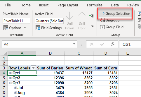
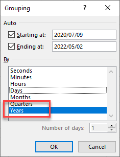
5. To change the way that the pivot table groups, select the row field in the pivot table and then, in the Ribbon, go to Pivot Table Analyze > Group > Group Selection.

 

 

6. Choose the grouping you wish to show. For example, you may just want Months and Days.

 

 

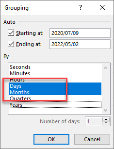
7. This would remove the year, though – so any orders on the 1st of May, for example, are on that day – regardless of the year of the order!

 

 

8. If you only include one option in the grouping, the ability to drill down is removed.

 

 

9. You can, however, then select the field in the pivot table, and then click again on Group Selection in the Ribbon to add other grouping options back.

 

 

Ungroup Data

You may wish to remove groups that have been created in your pivot table.

Click in a field in your pivot table that is part of a group and then, in the Ribbon, go to PivotTable Analyze > Group > Ungroup.

 

 

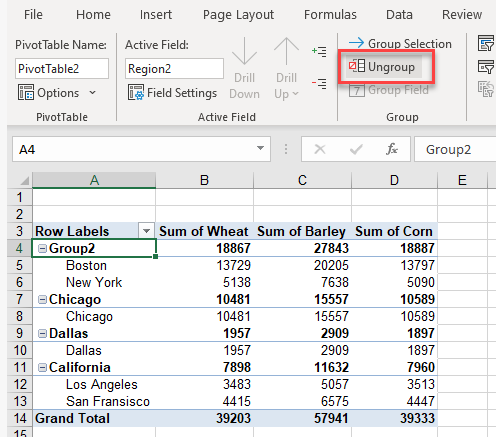
The grouping for that field is removed.

 

 

Pivot Table Filters

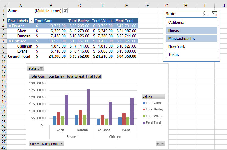
When you add field to a pivot table, Excel automatically adds filter buttons.

 

 

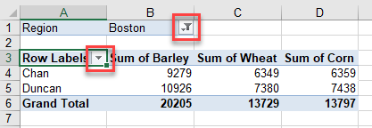
1. Click on any of the (Region) items to filter your pivot table by one of the values found in that list.

 

 

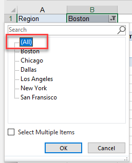
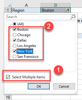
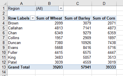
2. To clear the filter from the Region field, click on the filter button, and then click on (All). Click OK.

 

 

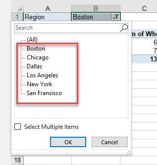
3. To filter by more than one value, tick Select Multiple Items and then choose the items to filter for. Click OK to apply the filter to your pivot table.

 

 

Create and Use Slicers With Pivot Tables

Slicers are another way to filter a pivot table.

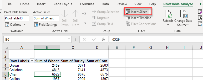
1. In the Ribbon, go to PivotTable Analyze > Filter > Insert Slicer.

 

 

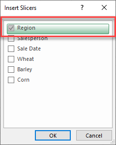
2. Select the field you wish to insert a slicer for, and then click OK.

 

 

All of the available data options are automatically shown.

 

 

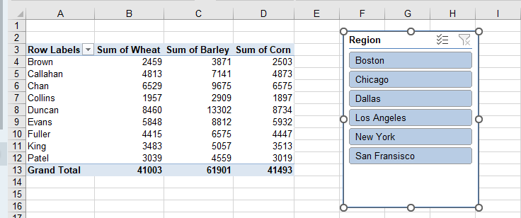
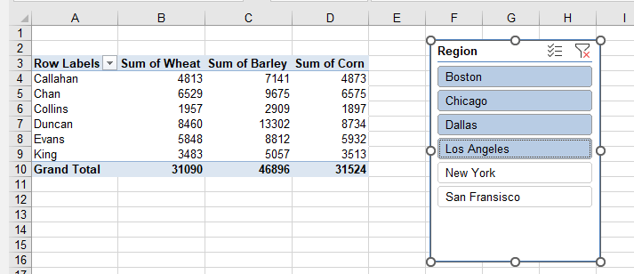
3. Click on the top value (e.g., Boston), and then hold down the CTRL key to select any additional values. The pivot table updates dynamically to reflect the filter.

 

 

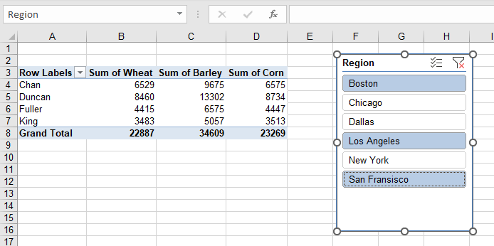
4. If you want to select adjacent values, click on the first value in the slicer, and then holding down the SHIFT key, click on the final value you need.

 

 

5. To remove the slicer, click on it and press the DELETE key. This also removes any filtering that the slicer applied to your pivot table.

Format Pivot Table Values

When you create a pivot table, the values are formatted as a general number format.

 

 

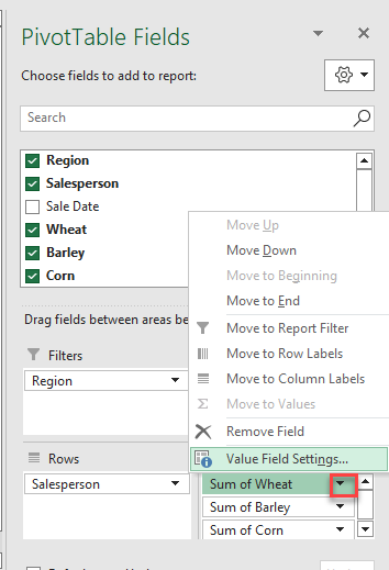
To format the numbers, it is best to use the formatting options in the PivotTable Fields Values box.

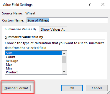
1. In the small drop down next to the field in the Values box, click Value Field Settings…

 

 

2. Then click Number Format.

 

 

3. Choose from the Category list, and then click OK to apply the format to the relevant field.

 

 

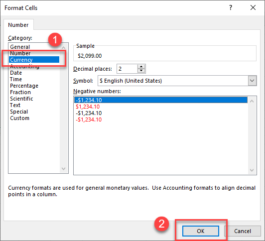
4. Click OK again to return to the PivotTable Fields list.
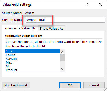
   At this stage, you can also change the name of the label that is displayed in the pivot table.

 

 

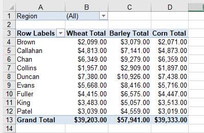
5. Repeat the steps above for the rest of the fields where you want to apply a number format.

 

 

Hide and Unhide Pivot Table Subtotals

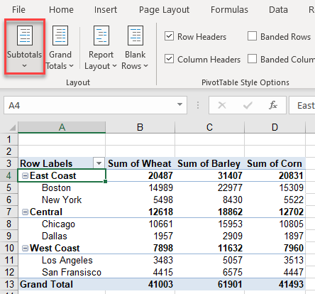
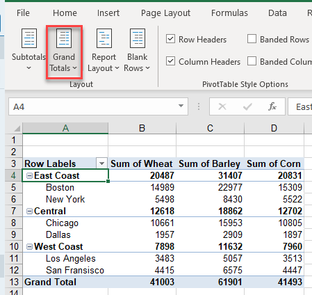
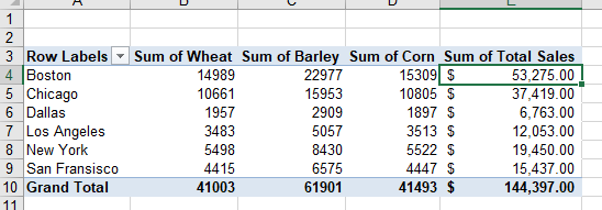
By default, there’s a Grand Total at the bottom of a pivot table; if you have grouping applied, subtotals are also added for each group.

To remove subtotals:

1. In the Ribbon, go to Design > Layout > Subtotals.

 

 

2. Click Do Not Show Subtotals.

 

 

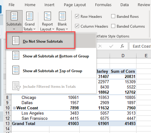
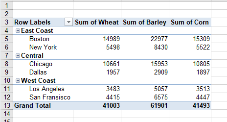
Any subtotals are removed from the pivot table.

 

 

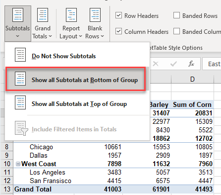
You could also set the subtotals to show at the top or bottom of each group.

 

 

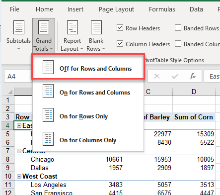
3. To show or hide the Grand Total, in the Ribbon, go to Design > Layout > Grand Totals.

 

 

4. Choose which option you want for Grand Totals. For example, to hide all grand totals, click Off for Rows and Columns.

 

 

Pivot Table Calculated Fields

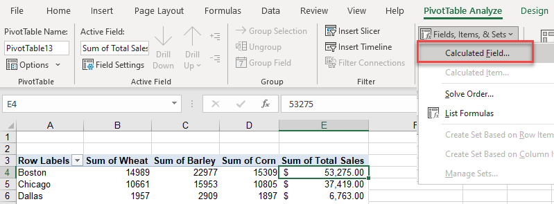
You can add calculated fields to your pivot table.

1. In the Ribbon, go to PivotTable Analyze > Calculations > Fields, Items & Sets > Calculated Field.

 

 

2. In the Name field, type in the name for the field, and then in the Formula box, type in the formula for your new field. Click Add to have the new field included in the Fields list below.

 

 

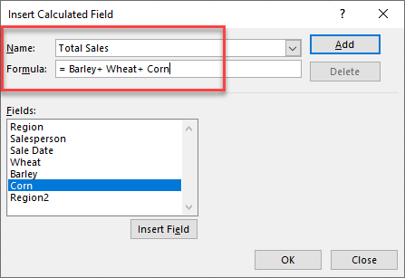
3. Click OK to add the field to your pivot table.

 

 

Move Pivot Table

When you create a pivot table, you are given the option (if you do not use a recommended pivot table) to insert the pivot table either into a new sheet, or into the sheet where you are currently working.

If you change your mind about placement, you can always move the table after it’s been created.

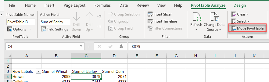
1. In the Ribbon, go to PivotTable Analyze > Actions > Move Pivot Table.

 

 

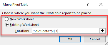
2. Choose where you want the pivot table to be placed. In this example, move the existing pivot table to the Sales Data worksheet.

 

 

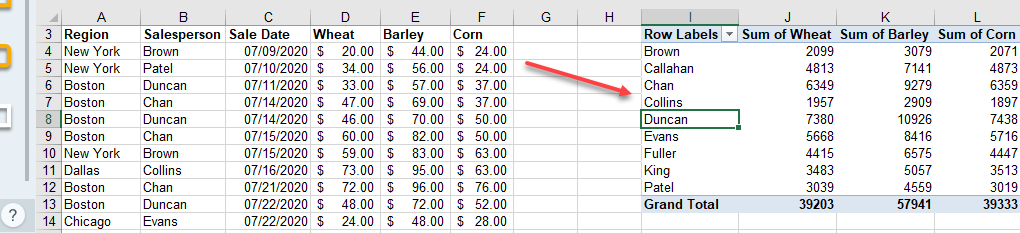
3. Click OK to move your pivot table.

 

 

Insert Pivot Chart

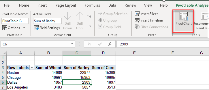
You can create a chart based on your pivot table.

1. Click on your pivot table, and then, in the Ribbon, go to PivotTable Analyze > Pivot Chart.

 

 

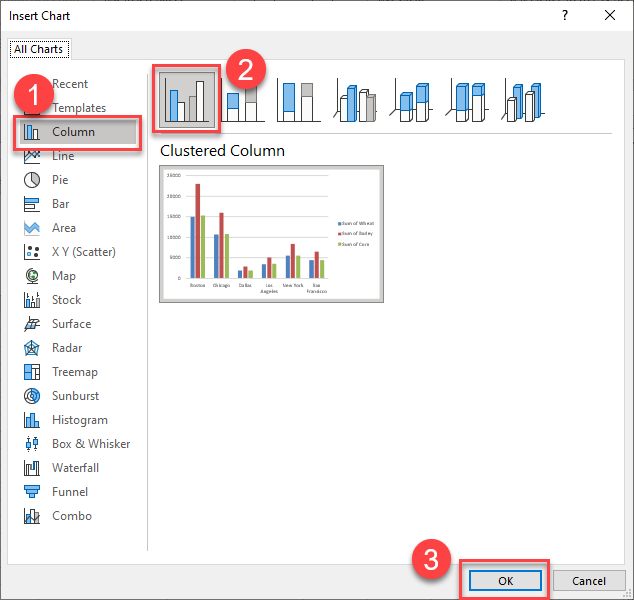
2. In the Insert Chart dialog box, choose the kind of chart and then choose the Style. Finally, click OK to insert the chart into your worksheet.

 

 

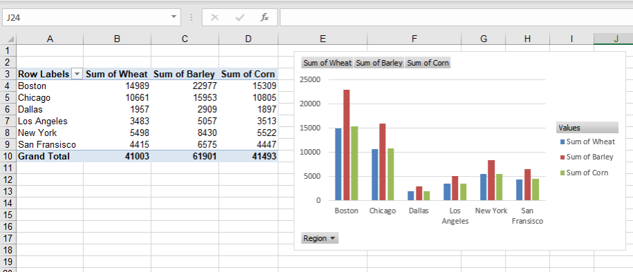
3. A chart is placed in your worksheet. To move the chart, click in the middle of the chart so the cursor changes to a small black cross. Then drag your chart to the desired location.

 

 

Pivot Table Default Options

Table Options

There are a number of default settings that are set when you create a pivot table. You can change these options in PivotTable Options.

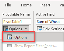
1. Click in your pivot table and then, in the Ribbon, go to PivotTable Analyze > PivotTable > Options.

 

 

2. Change the PivotTable Name in the first field if you need to. This could prove useful if your file has multiple pivot tables.

 

 

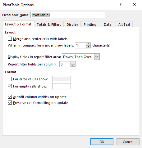
3. Click on the tab you need, and then set the options in that tab for the pivot table.
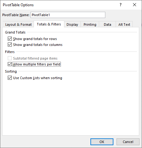
   In the Totals & Filter tab, for example, you can switch grand totals on or off for rows and columns. Tick Allow multiple filters per field to make this the default option for your pivot table.

 

 

Pivot Table Styles

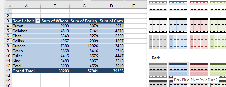
When you create a pivot table, a default style is automatically applied. You can change the table style to alter the appearance of your pivot table.

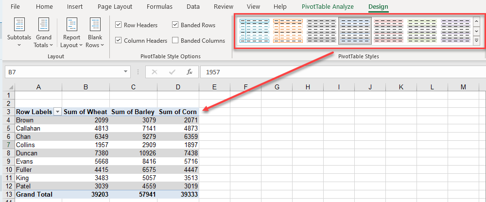
Apply a Pivot Table Style

1. Select the pivot table, and then in the Ribbon, go to Design > PivotTable Styles. Click the up or down arrows to show preset style options in the style box. Then click on the style you want.

 

 

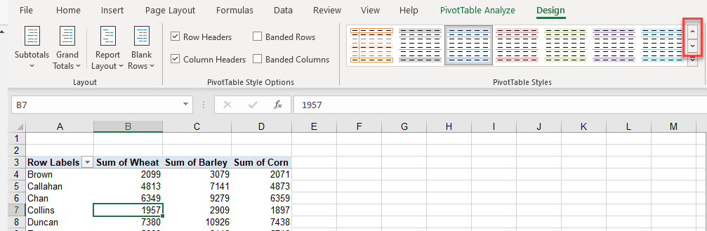
2. Alternatively, to see more styles, click the More button (the bottom down arrow).

 

 

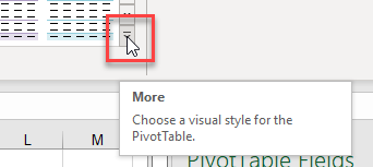
This brings up a list of available styles.

 

 

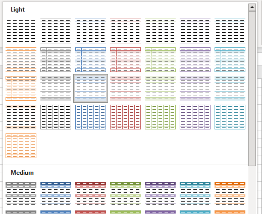
3. Choose the one you want to apply it to your pivot table.

 

 

Create Custom Style

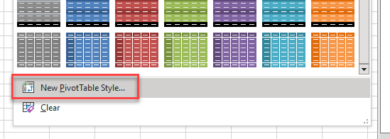
You can also create a custom style.

1. At the bottom of the list of styles, click New PivotTable Style.

 

 

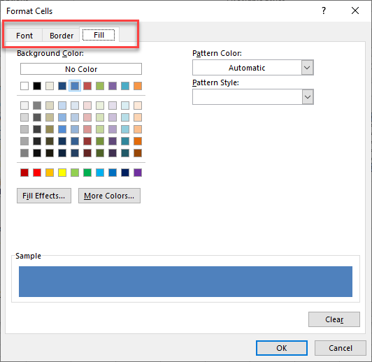
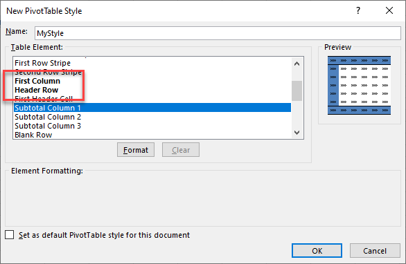
2. In the Name field, type in the name for your style and then in the Table Element list, choose the part you wish to format. Click Format.

 

 

3. Adjust the font, border, and/or fill formats, and then click OK.

 

 

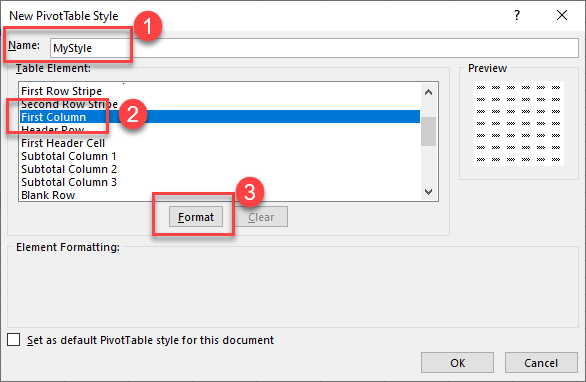
4. Notice that in the Table Element list, the elements you have formatted are now bold. A preview of your style is shown on the right side of the box. Click OK to add your new style to the Styles list.

 

 

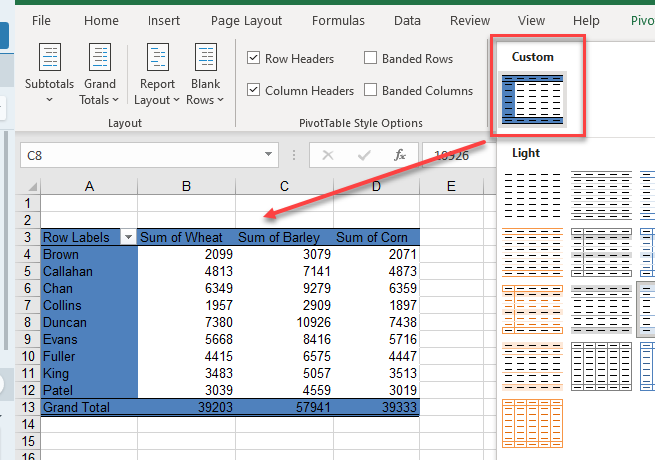
5. Click in the PivotTable Styles box and choose a custom style to apply to your pivot table.

 

 

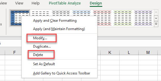
6. To modify or delete a custom style, right-click it and choose another style option.

 

 

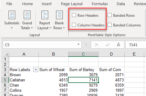
Style Options

When you apply a pivot table style, a number of default options are automatically applied, such as Row Headers and Column Headers. In the Design tab, PivotTable Style Options group, you also have Banded Rows and Banded Columns available.

 

 

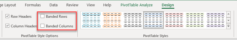
1. To apply the row formatting, tick the Banded Rows box. Notice that the preview in PivotTable Styles shows the rows being formatted with alternating colors for all the styles, while the style that is currently applied to your pivot table formats your pivot table with these colors.

 

 

2. Tick the Banded Columns box to also apply the column formatting to your pivot table.
3. You can also use the style options to remove formatting on Row Headers and Column Headers.

 

 

Advanced Pivot Table Techniques in Google Sheets

Pivot tables in Google Sheets are not as advanced as those in Excel. You can change the data range, and you are able to add a filter to your pivot table.

Update or Change the Data Range

1. Make sure your cursor is on a cell within the pivot table, and then in the Pivot table editor, click the Select data range button.

 

 

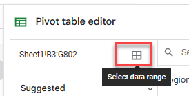
2. Click in the box with the selected range. You can then select the range of data that you wish the pivot table to be based on.

 

 

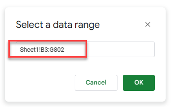
3. Click OK to apply the new or updated range to the pivot table.

Add Filter

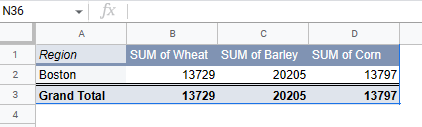
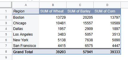
Consider the following Google Sheets pivot table.

 

 

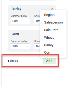
1. In the pivot table editor, click the Add button next to Filters, and then choose the field you wish to filter by (e.g., Region).

 

 

2. Click clear to uncheck all values, and then tick the value to filter for. Click OK.

 

 

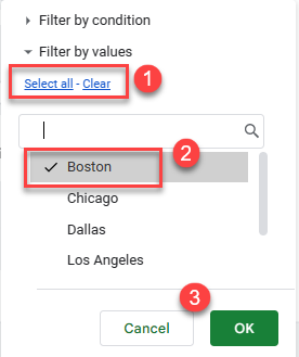
The chosen filter is applied. Here, only data from the Boston region is included in the table.