Remove a Field From a Pivot Table in Excel & Google Sheets
Written by
Reviewed by
This tutorial demonstrates how to remove a field from a pivot table in Excel and Google Sheets.
Remove Pivot Table Field
When you have a pivot table in Excel, each field is associated with a column from the source data. To simplify or further summarize your pivot table, you might want to remove one of the fields. There are a few ways to do this.
Remove Field From PivotTable Fields List
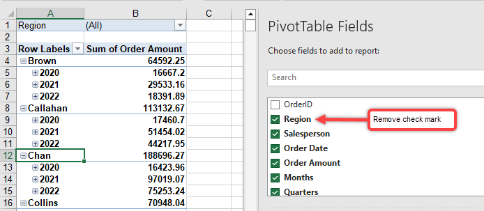
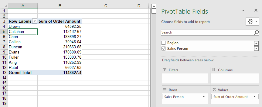
The fields displayed in your pivot table are checked in the PivotTable Fields list. Simply uncheck a field to remove it from the pivot table. However, if your field is a date, double-check for automatic date fields that may have been created.
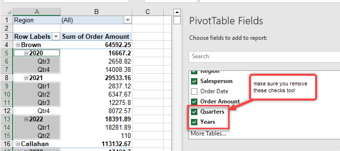
When you add a date field to a pivot table, it creates two new fields – Quarters and Years – that are automatically added to the table. To completely remove a date field from the pivot table, you have to remove all the date fields: the original field and the automatically generated fields.
Drag the Field Off the Layout Grid
You can remove a field from your pivot table by dragging the field off the list. For this example, remove the Region field from the Filters area.
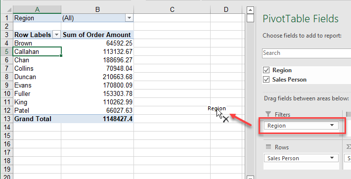
Select the field and drag it off the Field List with your mouse. Note that, since the Regions filter was already set to (All), the Order Amount values don’t change.
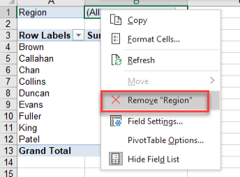
Right-Click the Field
Finally, you can remove a field by right-clicking on the field in the pivot table itself and clicking Remove “Region“ (where the text in quotes is the field name).
Tip: Try using some shortcuts when you’re working with pivot tables.
Remove a Pivot Field in Google Sheets
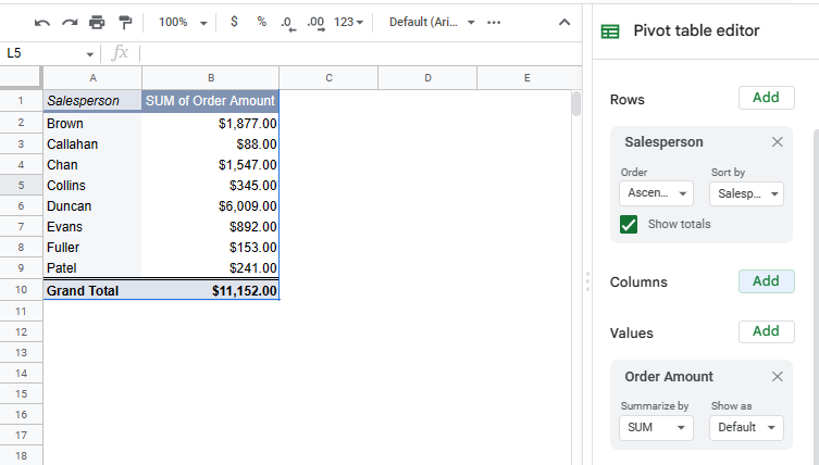
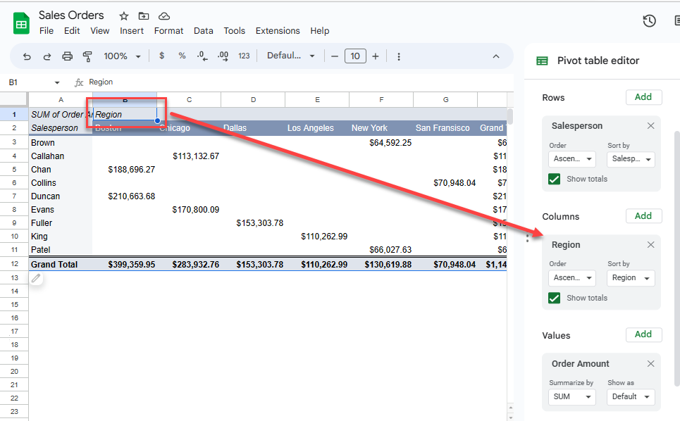
Consider the Google Sheets pivot table below.
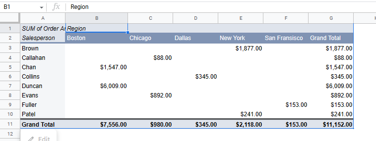
It’s been set up with Region as the Columns field, Order Amount for Values, and Salesperson as the Rows field.
▸ To remove the Region field, in the Pivot table editor, click the cross in the top-right corner next to the field name.
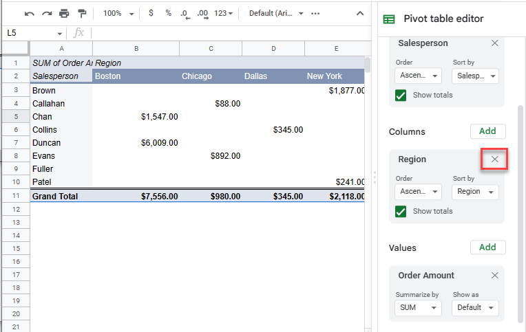
The pivot table is updated to reflect the changes, and Order Amount sums are split only by Salesperson.