How to Keep Formatting on a Pivot Table in Excel & Google Sheets

This tutorial demonstrates how to keep formatting consistent on a pivot table in Excel and Google Sheets

 

 

Pivot Table Field Number Format

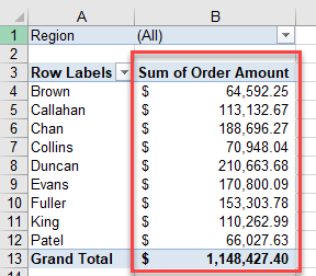
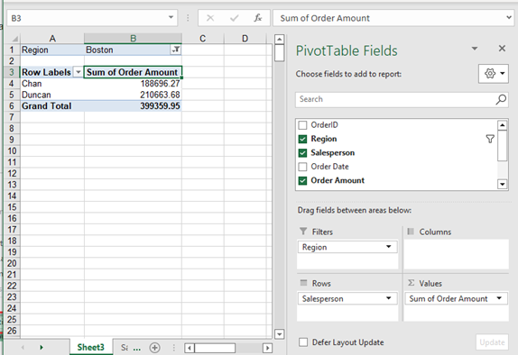
Pivot tables are a great for displaying simplified data from a searchable database in Excel. But a few extra steps are necessary when you want to add formatting to a pivot table. Consider the following pivot table.

 

 

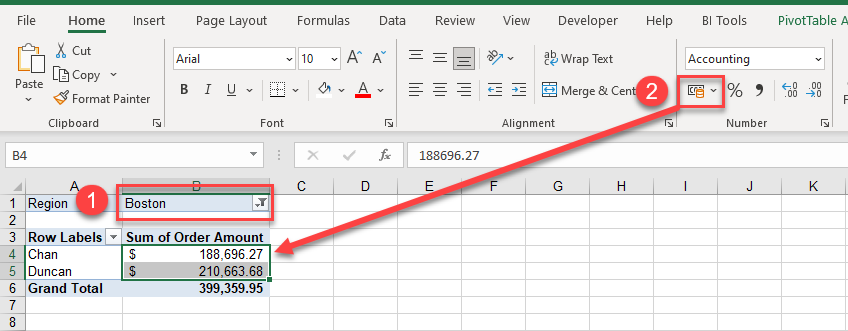
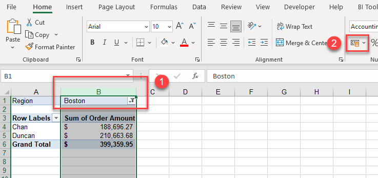
In the example below, there’s a filter on (1) Region, and the figures in the Sum of Order Amount field are (2) formatted using the Accounting Format button in the Ribbon.

 

 

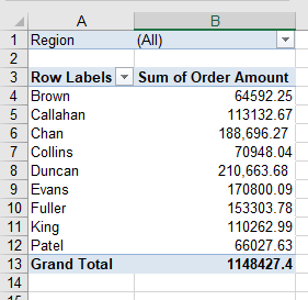
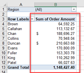
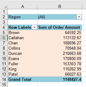
However, if you remove the filter from Boston, the rest of the rows in the pivot table are not formatted with the currency symbol!

 

 

To ensure that all the value rows are formatted correctly, set the number format of the actual field in the pivot table.

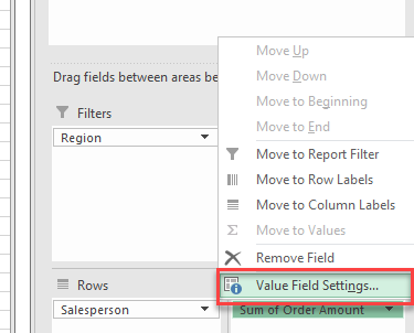
1. Click in the pivot table. This brings up the PivotTable Fields pane on the right side of the window.

 

 

2. In the PivotTable Fields pane, click Value Field Settings… on the Values field drop down.

 

 

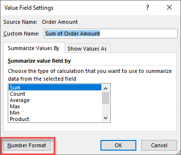
3. Click Number Format.

 

 

4. Select Accounting from the Category list, and then pick the appropriate currency symbol from the Symbol drop down.

 

 

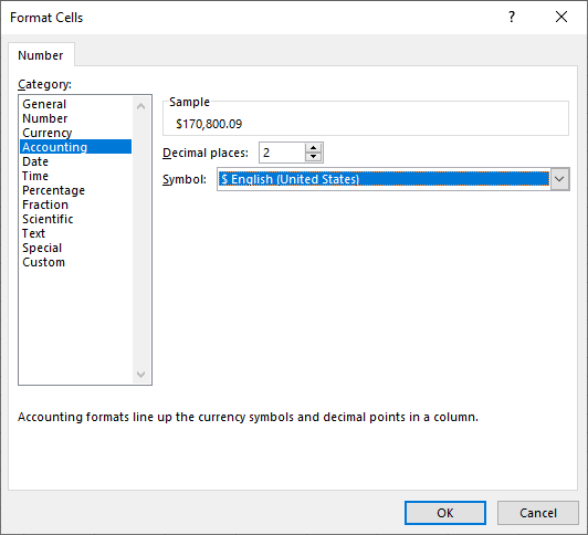
5. Click OK, and then OK again to return to Excel and apply the formatting to all the value fields in the pivot table. Now if any data is added to the pivot table, the value field retains the format applied.

Format a Column of Data

You can also format the entire column of data that a value field is using in a pivot table.

1. Select the entire column (not just the range B4:B6) by clicking on the column header.
2. Apply the format.

 

 

3. Remove the filter to check that the formatting was correctly applied. As you can see below, rows that had been hidden all have the same format.

 

 

Preserve Format on Update

Look at the pivot table below. It has been formatted with different background colors.

 

 

Now, if you wish to refresh the pivot table to update the data, you can, in the Ribbon, go to Data > Queries & Pivots > Refresh All.

 

 

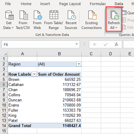
As you can see in the above example, all the custom background formatting has been removed and the default colors are reapplied!

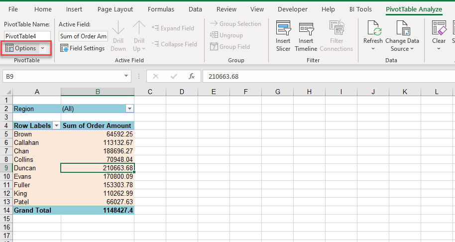
1. To prevent this from happening (and to keep the custom colors!), in the Ribbon, go to PivotTable Analyze > PivotTable > Options.

 

 

2. Tick Preserve cell formatting on update and click OK.

 

 

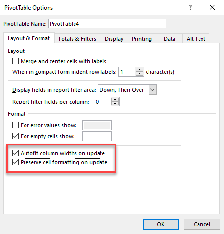
3. If you also changed the column widths in your pivot table, uncheck Autofit column widths on update to ensure you preserve your custom column widths.

Tip: Try using some shortcuts when you’re working with pivot tables.

How to Keep Formatting on a Pivot Table in Google Sheets

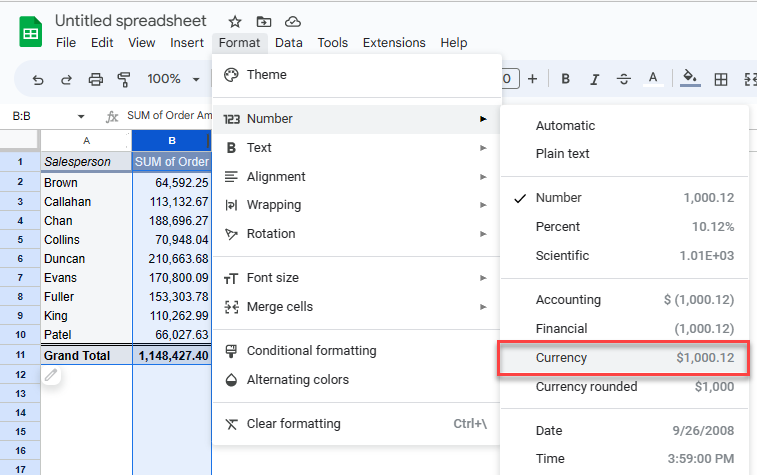
You can format data in a pivot table in Google Sheets by formatting the column or cells that contain the data. Select the cells in the pivot table, and then in the Menu, go to Format > Number. Choose a format that suits your needs (e.g., Currency).

 

 

This applies the chosen formatting to your pivot table column.

 

 

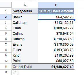
If you remove the pivot table field (here, Order Amount) from that column and add a different field, the formatting remains.