How to Change Data Source Reference for a Pivot Table in Excel and Google Sheets

This tutorial demonstrates how to change the data source reference for a pivot table in Excel and Google Sheets.

 

 

Whenever you have a pivot table, it is based on a dataset in the same sheet, a different sheet in the workbook, or even in another file. When the source data changes, you can sometimes simply refresh the associated pivot table(s).

Other times, the address of the source has changed or the source data has been expanded. Then, it’s necessary to change the data source directly in the pivot table.

Change Data Source Manually

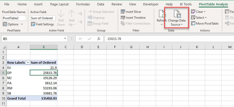
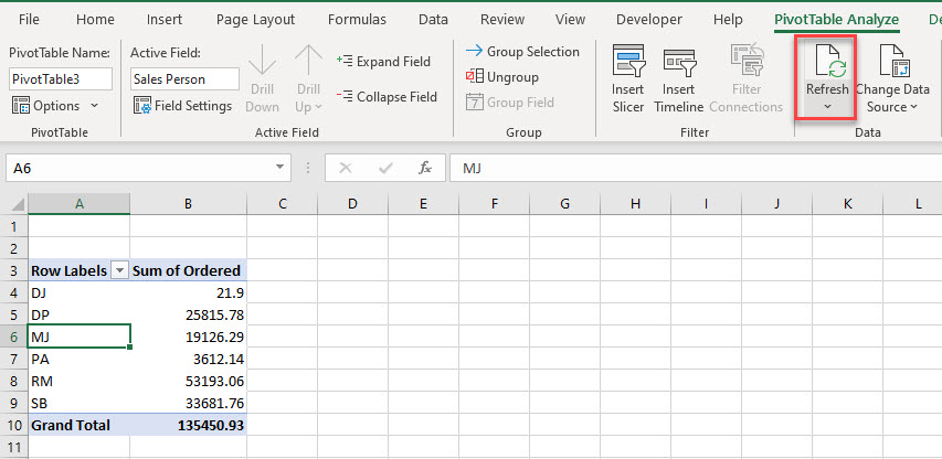
1. Click within your pivot table in order to show the PivotTable Analyze tab in the Ribbon.
2. In the Ribbon, go to PivotTable Analyze > Data > Change Data Source.

 

 

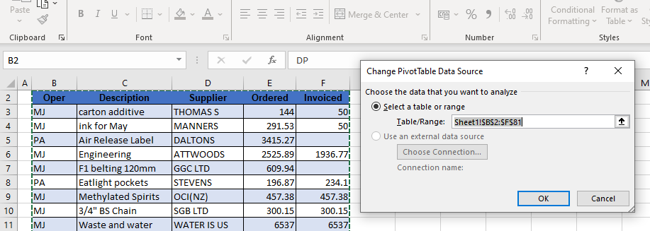
3. Click the small arrow to the right of the existing range that is already entered in the Table/Range box.

 

 

4. Select the new range of cells for your pivot table and then click on the small arrow to the right of the selected range address.

 

 

5. Click OK to change the data source.

Change the Data Source Automatically

If your data is set up as an Excel table, and you add data to this table, the data source for your pivot table is automatically updated to include any extra data that is added to your table.

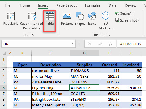
1. Before you create a pivot table, click within your data, and then, in the Ribbon, go to Insert > Table.

 

 

2. Your entire data area should be selected as long as there are no blank cells, rows or columns in the data area.

 

 

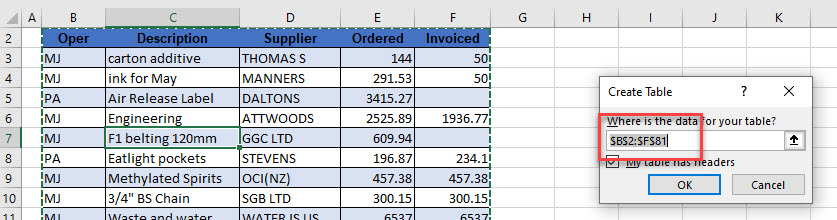
3. Click OK to create your table.
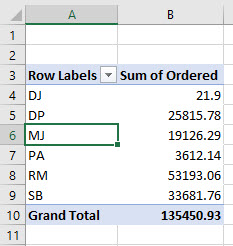
4. Now, create a pivot table by clicking in the middle of the table of data, and in the Ribbon, go to Insert > Pivot table. Add to the column, row, and value areas.

 

 

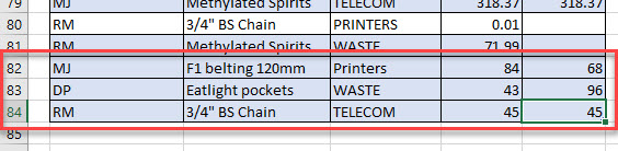
5. Next, go back to your data table, and add three more rows to the bottom of the data.

 

 

6. Switch back to your pivot table, and in the Ribbon, go to PivotTable Analyze, Change Data Source. Notice that the data source for your pivot table does not show a range of data, but rather the name of the table – in this case, Table1.

 

 

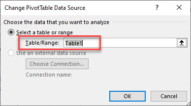
7. Therefore, you do not need to change the data source. The three new rows are automatically added.
   Instead, click Cancel and then, in the Ribbon, go to PivotTable Analyze > Refresh. This refreshes the pivot table to include the data from the new rows.

 

 

Data Source Reference is Not Valid

If you are changing the data source of a pivot table, and get the following message, it may be that your data source has been deleted or moved by mistake.

 

 

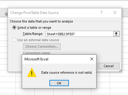
If this is the case, make sure that the table/range in the Select a table or range box is a valid range.

Tip: Try using some shortcuts when you’re working with pivot tables.

Change Pivot Table Data Source in Google Sheets

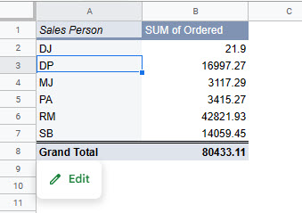
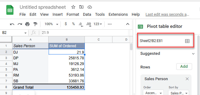
Consider the following pivot table:

 

 

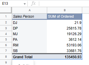
The data source is shown in the Pivot table editor.
If you cannot see the editor, click the Edit button at the bottom of the pivot table.

 

 

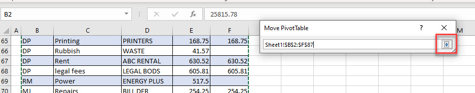
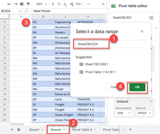
1. Click the Select data range button (⊞) to show the Select a data range box.

 

 

2. Then, select the data source range, click on the sheet that contains your source data and select the entire range.
   Finally, click OK to update your pivot table.

 

 

Pivot table values update accordingly.