How to Create a Pivot Table in Excel & Google Sheets

This tutorial demonstrates how to create a pivot table in Excel and Google Sheets, and how to work with pivot tables.

 

A pivot table summarizes a large tables of data, making it easier to view and analyze that dataset. Pivot tables are easy to build and edit, and they do your calculations for you.

Tips

• See how to create a searchable database and how to clean up your data in Excel. Those tutorials can help you avoid errors in translating a dataset to a pivot table.
• Try using some shortcuts when you’re working with pivot tables.

Create a Pivot Table

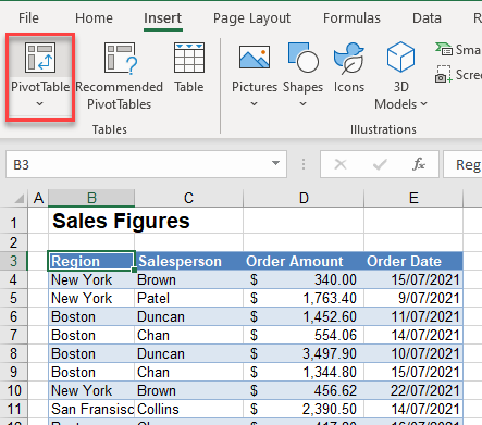
1. Click anywhere within the source data that you want to summarize in a pivot table.
2. In the Ribbon, go to Insert > Tables > Pivot Table.

 

 

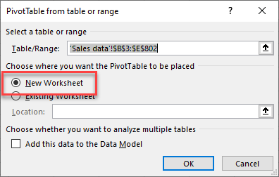
3. For Choose where you want the PivotTable to be placed, leave the default New Worksheet. (You can always move it later.)

 

 

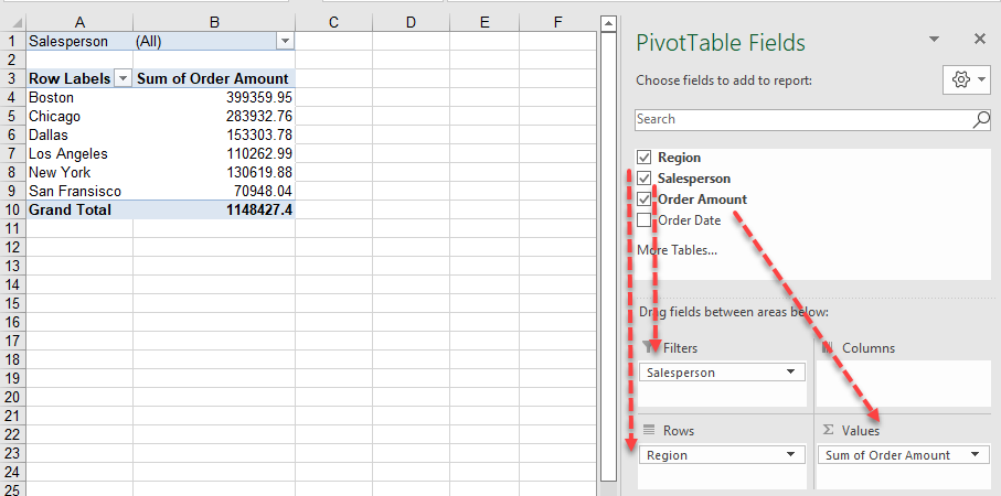
This inserts a new sheet with a blank pivot table. There are two new tabs added to the Ribbon: PivotTable Analyze and Design. On the right side of the screen, there’s a PivotTable Fields task pane showing your source data’s columns (fields).

 

 

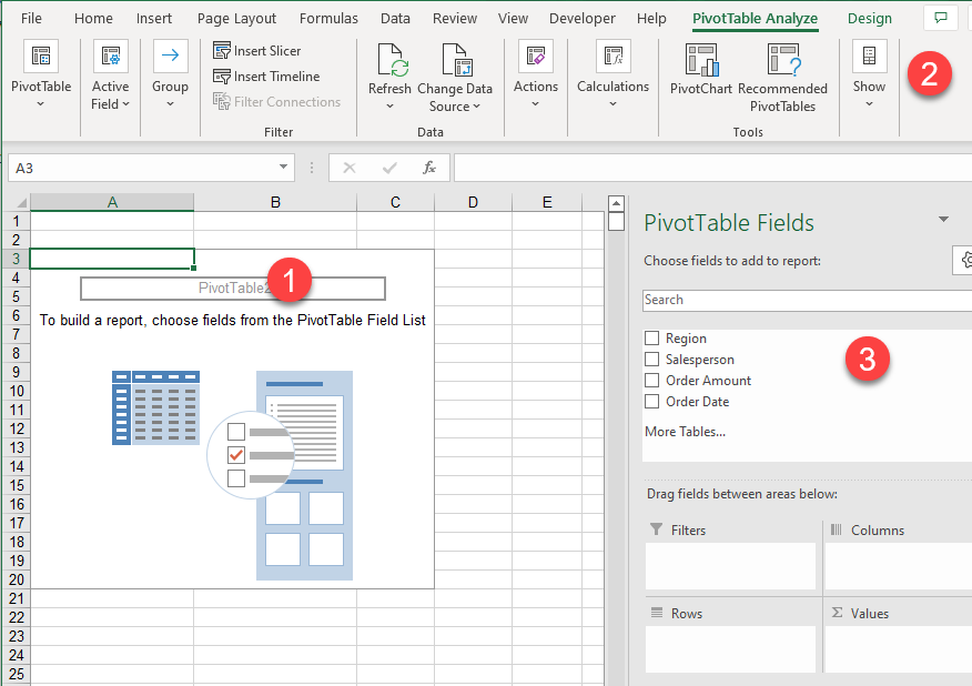
4. Drag each field you want to include down to the relevant section of the pivot table.
   For this example, drag Salesperson to the Filter section, Region to the Rows section, and Order Amount to the Values section.
   You can play around with the fields and drag them between rows, columns, and filters. (Note that anything dragged to Values that is not a number will automatically be counted rather than summed.)

 

 

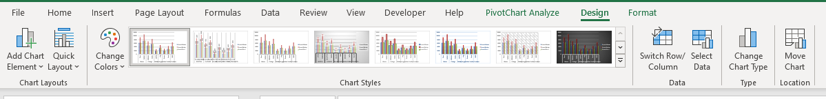
5. Now, to format the pivot table, use the Design tab. Go to PivotTable Styles and choose one of the styles shown. (Pivot table styles are similar to Excel’s Format as a Table options.)

 

 

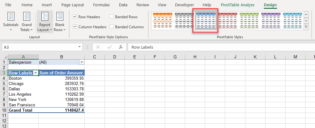
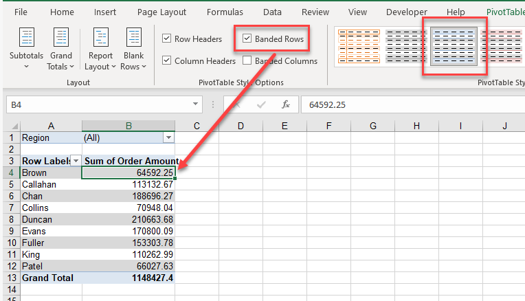
6. To customize your pivot table beyond the basic template, go to the PivotTable Style Options group. This allows you to toggle various elements on and off.

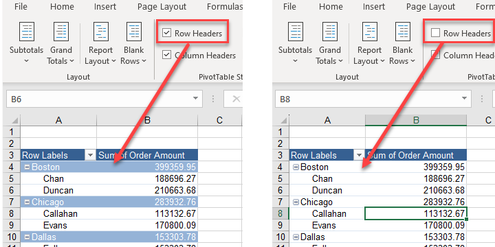
• The Row Headers checkbox switches row header formatting on and off. This can make field names easier to identify, especially when there are groups. Formatting applied to row headers is based on the style you chose in Step 5.

 

 

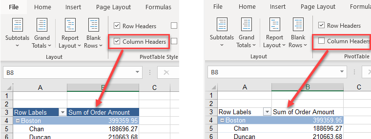
• Similarly, the Column Headers checkbox switches formatting for column headers on or off.

 

 

• If the Banded Columns and Banded Rows checkboxes are ticked, then each alternate column or row is formatted according to the style applied in Step 5. In the example below, Banded Rows is ticked, so color is applied to alternate rows.

 

 

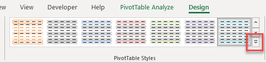
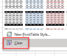
7. To clear formatting, in the Ribbon, go to Design > PivotTable Styles. Click on the small down arrow in the bottom-right corner of the Styles group.

 

 

8. Scroll down to the bottom and click Clear.

 

 

Work With Pivot Tables

Now that your pivot table is set up, there are a few important commands you should be familiar with.

Refresh a Pivot Table

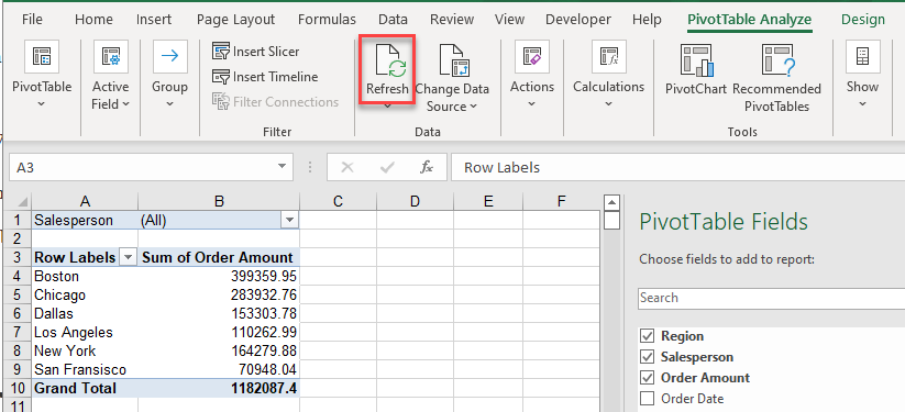
If the underlying source data changes, you need to refresh your pivot table to update the values.

In the Ribbon, go to PivotTable Analyze > Data > Refresh.

 

 

Delete a Pivot Table

1. In the Ribbon, go to PivotTable Analyze > Select > Entire PivotTable (or press CTRL + A while any cell in the table is selected).

 

 

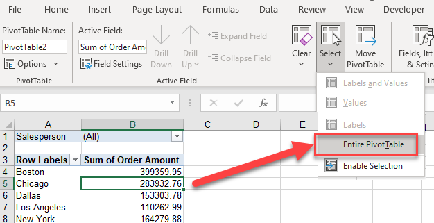
2. Press the DELETE key to get rid of the selected pivot table. Note that this only deletes the pivot table and not the underlying source data.

Filter and Sort in a Pivot Table

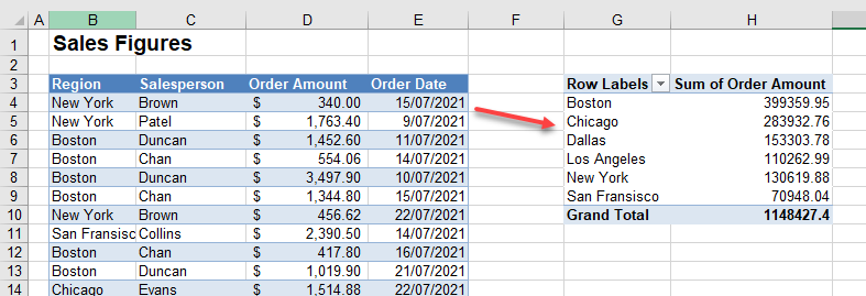
When you create a pivot table, Excel automatically adds filter buttons on Row and Column Labels, as well as any Filter field(s) at the top of the table. These automatic filters work similarly to Excel’s standard filtering.

 

 

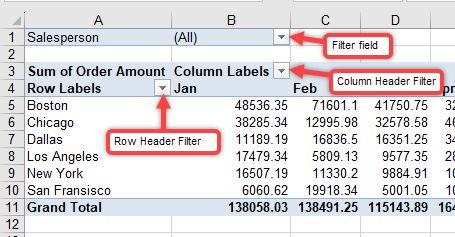
1. To filter a pivot table, click any of the filters’ drop downs (labeled in the picture above), and then tick the items to include.

 

 

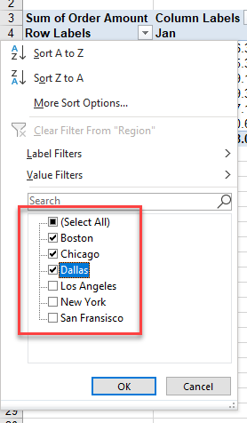
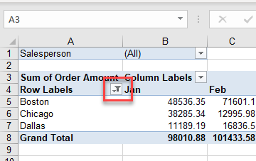
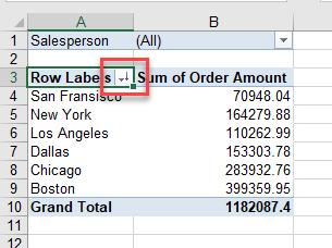
2. Click OK to show the filtered data. Notice that filter button(s) show a small funnel icon when a filter is applied, indicating that some data is filtered out and hidden.

 

 

3. The filter drop down lets you sort the data in addition to filtering the data. You can sort the data that has already been filtered, or sort the data unfiltered. To sort the data alphabetically, click Sort A to Z.

 

 

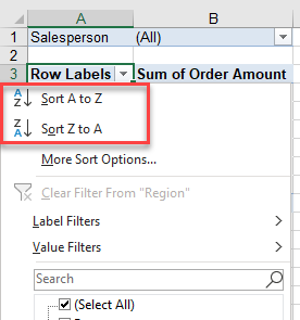
4. Click Sort Z to A to reverse the order of the data. Notice that, once you have done this, a small arrow in the direction of the sort appears on the filter button.

 

 

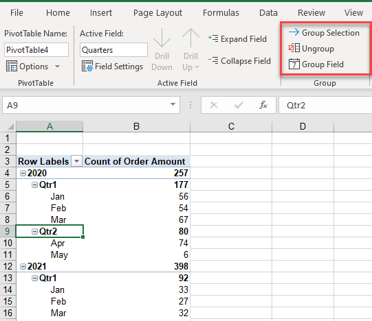
Group Pivot Field Items

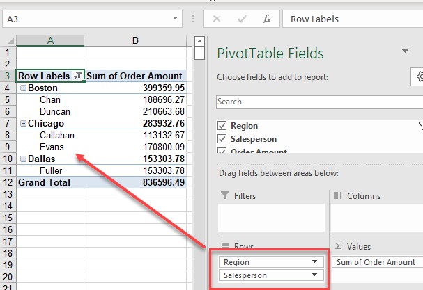
Grouping related rows or columns together is a popular feature in Excel. If you add two or more fields to the Rows and/or Columns sections (or a date field), Excel automatically groups those fields.

1. Add two fields to the Rows section. The second field added is grouped under the first field.

 

 

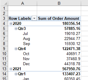
For date fields, the pivot table adds grouping automatically. Dates are grouped by year, quarter, and month.

 

 

2. To customize groups, click Group Selection or Ungroup in the PivotTable Analyze tab.

 

 

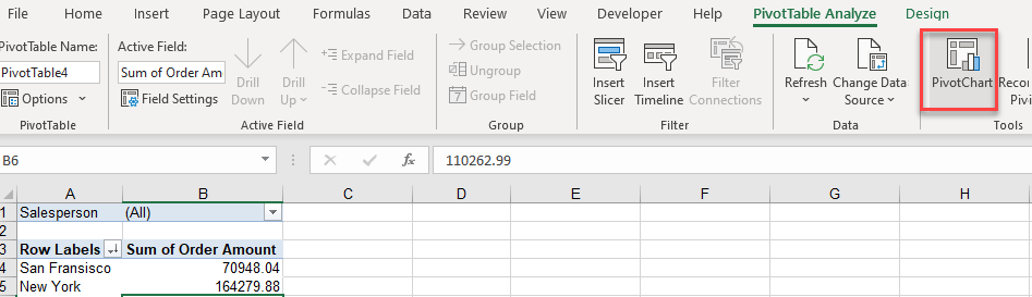
Create a Pivot Chart

1. To create a chart based on your pivot table, in the Ribbon, go to PivotTable Analyze > Tools > PivotChart.

 

 

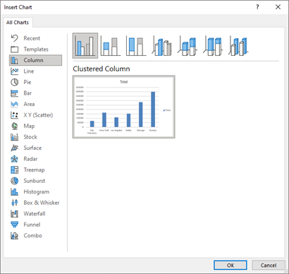
2. Choose the chart type you want, and then click OK.

 

 

3. Note that the PivotTable Analyze tab on the Ribbon is replaced with the PivotChart Analyze tab. The chart is the same as any other Excel chart, except that it has filters available on each field. For example, the chart below is filtered on Salesperson and Region.

 

 

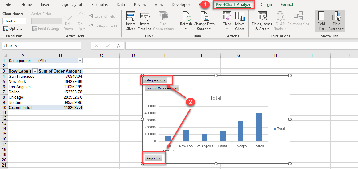
4. From the Design tab, customize the chart by choosing a different type, adding elements, or changing the colors.

 

 

Pivot Tables in Google Sheets

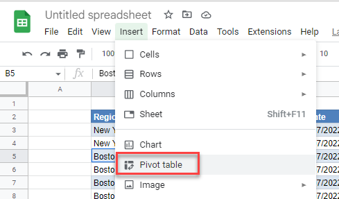
1. Click anywhere within the source data that you want to summarize in a pivot table. In the Menu, go to Insert > Pivot table.

 

 

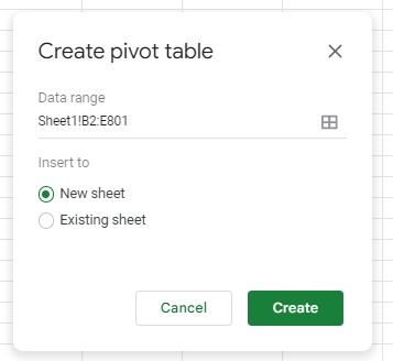
2. For Insert to, leave the default New sheet; then click Create. (You can always move it later.)

 

 

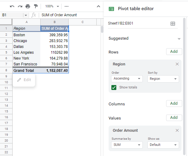
3. From the task pane on the right side of the screen, choose the fields to add to the rows, columns, and values sections. This step is similar to Excel.

 

 

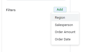
4. To create a filter, click Add in the Filters section and choose the field to filter by.

 

 

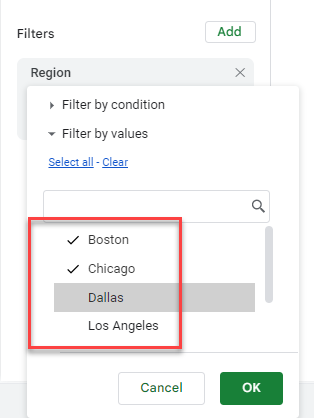
5. Tick the items to include in the pivot table (filtering out the unchecked items), and then click OK.

 

 

6. To delete a pivot table in Google Sheets, select all the columns and rows of the pivot table and press DELETE on the keyboard.

Notes

• A pivot table in Google Sheets automatically refreshes when the source data changes; it does not need to be manually refreshed.
• Sorting and grouping options available in Excel pivot tables are not available in Google Sheets, but the ability to filter data is.

More Pivot Table Tutorials

 

Pivot Tables
Add Calculated Field to Pivot Table
Advanced Pivot Table Techniques
Change Pivot Table Data Source
Count Unique Values With Pivot Table
Create Pivot Table
Delete Pivot Table
Filter Pivot Table Values
Get a Count in Pivot Table
Group Pivot Table by Date
Keep Pivot Table Formatting
Make a Pivot Table Chart
Pivot Table Slicers
Pivot Table Sorting Guide
Refresh a Pivot Table
Remove Field From Pivot Table
The Pivot Table Field Name Is Not Valid
Duplicates	yes
Distinct (Unique) Values
Shortcuts	yes
Pivot Table Shortcuts
Tables	yes
Create Table
Remove a Table or Table Formatting
Table Tools
Types of Tables
VBA	yes
Refresh Pivot Table When Data Changes
VBA Dynamic Range
VBA Guide to Pivot Tables
VBA Pivot Table Filter
VBA Refresh Pivot Table
VBA Runtime Error 5
VBA Turn Off AutoFilter