Work With Distinct / Unique Values in Excel & Google Sheets

This tutorial demonstrates how to work with distinct values in Excel and Google Sheets.

When you have a sheet of data in Excel that contains repetitive data, there are several methods you can use to isolate distinct values (or distinct rows) from your data. This tutorial covers five methods:

1. Formulas
2. Pivot Table
3. Conditional Formatting
4. Advanced Filter
5. VBA

It also shows how to count and select distinct values. Click here to jump to the Google Sheets section.

Formulas to Find Distinct Values

The UNIQUE Function

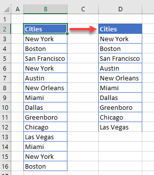
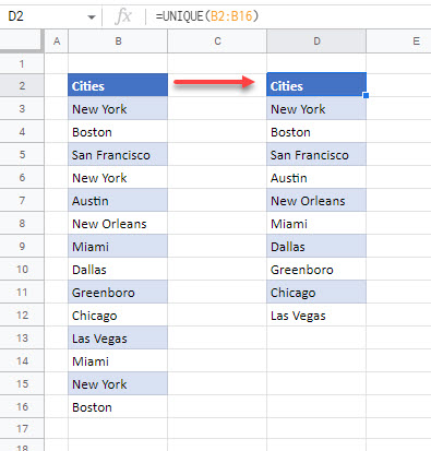
To extract unique values out of a list of values in Excel that contains duplicates, you can use the new UNIQUE Function. This function is only available in Excel 365. Consider the following list of values:

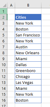
The list in Column B contains repetitive names of cities.

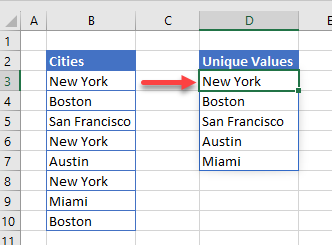
1. To extract the unique values from this list, click in D3 and type in the formula:

   =UNIQUE(B3:B16)

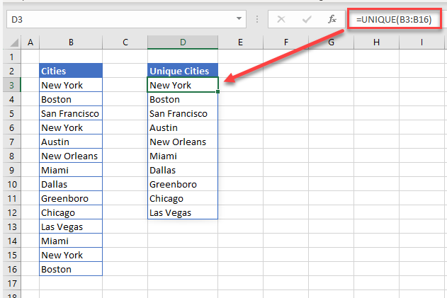
2. When you press ENTER, the formula populates the rows below with the unique values from Column B. (Any repeated cities are only shown once.)

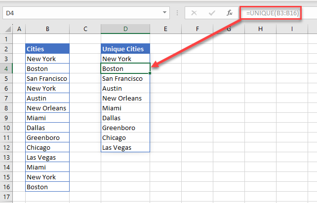
Notice that, if you move your pointer to cell D4, the formula in D4 is grayed out – you are not able to change it. This is because the list is automatically filled in by the formula contained in cell D3 – you can only edit or delete the formula if you have D3 selected. It’s an array formula.

Formulas Prior to Excel 365

If you’re not using Excel 365, there is no UNIQUE Function available. Showing unique values from a list with duplicates requires more work and a formula that uses four Excel functions: IFERROR, INDEX, MATCH, and COUNTIF.

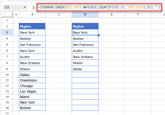
Use the formula below, where the original list in in Column B and the unique list is in Column D.

=IFERROR(INDEX(B$3:B$10,MATCH(0,COUNTIF(D$2:D2,B$3:B$10),0)),"")

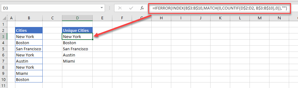
• The COUNTIF Function counts values that fit specified criteria. This section of the formula – COUNTIF(D$2:D2,B$3:B$10) –returns a zero for values that aren’t found earlier in the list. In other words, a zero result identifies each new item. Any other result means that the item is a duplicate and should be ignored.
• The MATCH Function . This section – MATCH(0,COUNTIF(D$2:D2,B$3:B$10),0) – returns the row number for each value with zero returned by COUNTIF. For example, the output for the MATCH portion of the formula in D6 is 7, because Row 6 is a duplicate.
• The INDEX Function . This section – INDEX(B$3:B$10,MATCH(0,COUNTIF(D$2:D2,B$3:B$10),0)) – returns the value in the row number returned by MATCH. So, D6 shows the value in Row 7 of the original list (Austin).
• The IFERROR Function returns a blank if the formula extends to a cell outside the list range. This ensures you don’t get the #N/A error.

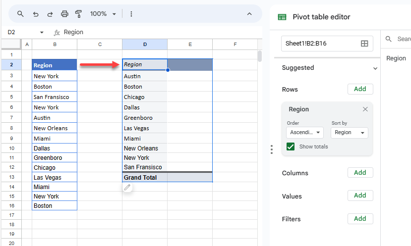
Pivot Table to Find Distinct Values

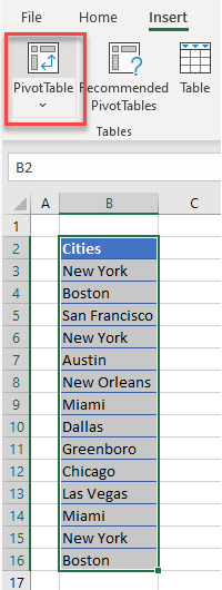
1. As with other methods in working with unique records, select the range of cells you want to obtain unique records from.
2. Then, in the Ribbon, go to Insert > Tables > Pivot Table.

3. Select a location in the Existing Worksheet to place your pivot table.

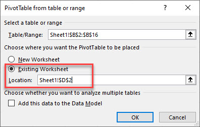
4. In the PivotTable Fields list, drag the field down to the Rows area of the pivot table.

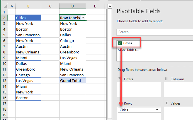
Pivot tables show only unique values.

Tip: Try using some shortcuts when you’re working with pivot tables.

Conditional Formatting to Find Distinct Values

You can use conditional formatting to find unique values in the data, and then you can filter by color to show just these values.

1. As with other methods in working with unique records, select the range of cells you want to obtain unique records from.
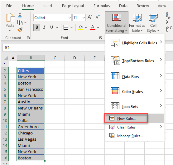
2. Then in the Ribbon, go to Home > Styles > Conditional Formatting > New Rule.

3. Choose Format only unique or duplicate values, and then in the Format all drop down, choose unique. Finally, set the format to be applied to unique cells.

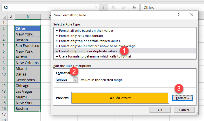
4. Click OK to apply the rule.

5. Now, in the Ribbon, go to Home > Editing > Sort & Filter > Filter and choose Filter by Color from the filter drop down.

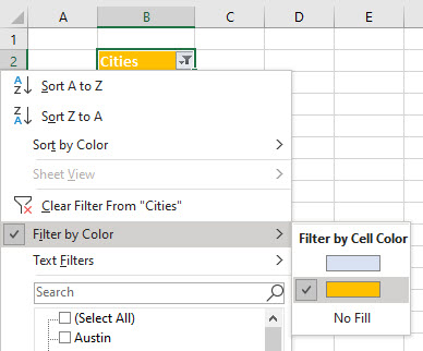
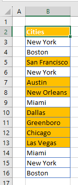
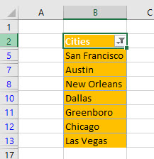
This filters out duplicate values, showing only unique ones in your worksheet.

Advanced Filter to Find Distinct Values

You can also use an advanced filter to find unique values.

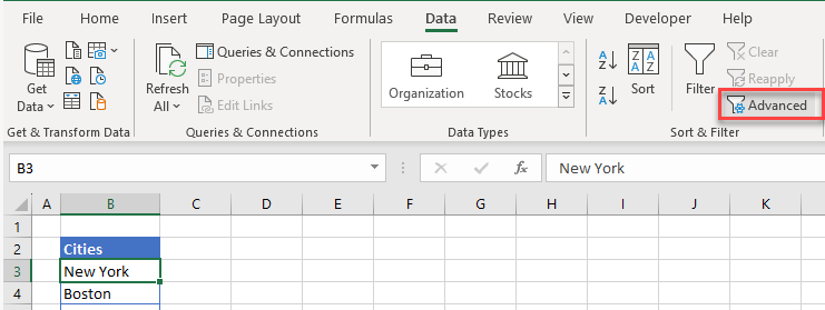
1. Select any cell in the list you wish to filter, and then in the Ribbon, go to Data > Sort & Filter > Advanced.

2. In the Advanced Filter dialog box, choose Copy to another location under Action. Then, type in or select the location you want to Copy to (i.e., where to place the filtered data). Finally, tick Unique records only.

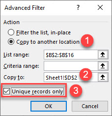
3. Click OK to filter for distinct records only.

VBA to Find Distinct Values

Finally, you can also find unique values using the RemoveDuplicates function in VBA.

Sub RemoveDups()
   Range("B2:B16").RemoveDuplicates Columns:=1, Header:=xlYes
End Sub

Distinct Values in Column vs Table

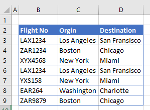
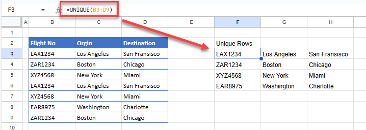
As shown at the beginning of this tutorial, the UNIQUE Function finds distinct values in a list (single column). It also works to find distinct rows in a table (multiple columns). Look at the table below. It’s a list of flight numbers and the corresponding origin and destination for each. Some rows are repeated.

To extract the unique rows, use the whole dataset range (B3:D9) as the array argument.

=UNIQUE(B3:D9)

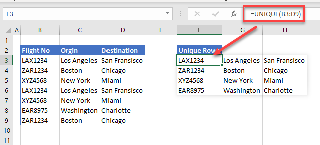
The UNIQUE Function populates a new set of unique data; there are just three columns instead of one.

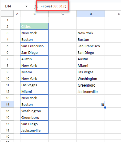
Count Distinct Values

Once you have extracted your distinct values, you can add a count to tell you how many distinct values or rows there are.

1. First, in a blank cell, type in the beginning of the ROWS Function:

   =ROWS(

2. Then, highlight the extracted unique rows (here, D3:D12).
3. When you press ENTER, the formula changes, showing a # sign at the end of the cell address.

   =ROWS(D3#)

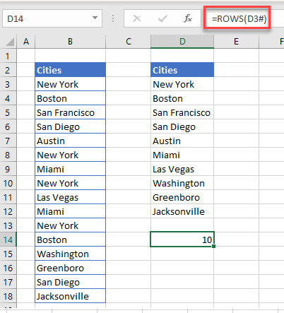
The formula returns a count of the unique values (rows) in the array.

Select Distinct Values

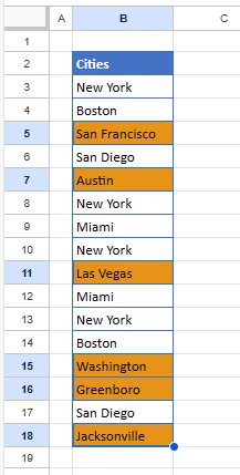
If you have used conditional formatting to filter by color to show distinct values, you can then select just these values using the Go To feature in Excel.

1. Highlight the list of data you filtered by color.
2. In the Ribbon, go to Home > Editing > Find & Replace > Go To Special…

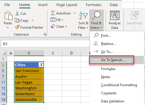
3. Choose Visible Cells only in the Go To Special dialog box.

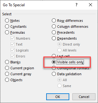
There are six distinct cities, and now the first instance of each is selected.

Distinct Values in Google Sheets

Find Unique Values

Google Sheets does not have VBA, but some of the methods used above (UNIQUE Function, alternate formulas, and pivot tables) can also be used in Google Sheets to obtain unique values.

• You can use the UNIQUE Function to extract values from a single column.

• You can also use the UNIQUE Function to extract unique rows.

• Unique values can also be extracted using a formula containing the INDEX, MATCH, and COUNTIF Functions.

• If you create a pivot table in Google Sheets, it automatically shows only unique values.

Count Distinct Values

Use the ROWS Function to count distinct values in Google Sheets.

Select Distinct Values

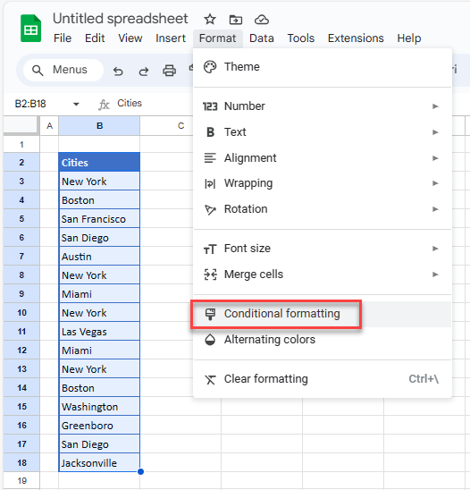
Use conditional formatting in Google Sheets to highlight – and then select – distinct values.

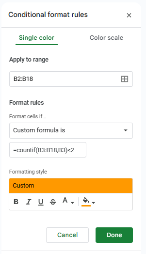
1. Highlight the list of data in which you wish to select the distinct values, and then in the Menu, go to Format > Conditional formatting.

2. Under Format rules, choose Custom formula is, and then type in the formula:

   =COUNTIF(B3:B18,B3)<2

3. Adjust the Formatting style, and click Done.

4. This applies formatting to distinct values in the list according to the custom format set in Step 3.

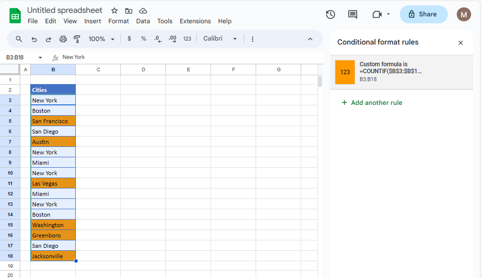
5. You can then easily select the highlighted values by clicking on the first highlighted value and then, holding down the CTRL key, click the rest of the highlighted values, one by one.