Lookup Min / Max Value – Excel, VBA, & Google Sheets
Written by
Reviewed by
Download the example workbook
This tutorial will demonstrate how to lookup min / max values in Excel and Google Sheets.
INDEX-MATCH with MIN
We can use the combination of INDEX, MATCH and MIN to lookup the lowest number.
=INDEX(B3:B7,MATCH(MIN(C3:C7),C3:C7,0))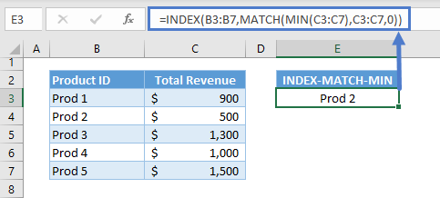
Let’s walkthrough the formula:
MIN Function
The MIN Function returns the smallest number from a list. It ignores non-numeric values (e.g., empty cells, strings of text, or, boolean values).
=MIN(C3:C7)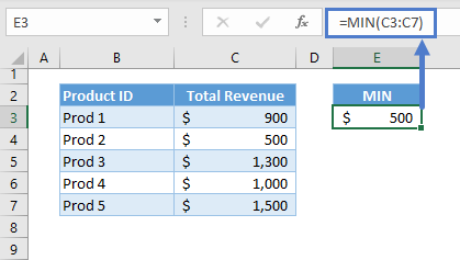
MATCH Function
Next, the result of the MIN Function is inputted as the lookup value for the MATCH Function in order to find the position or coordinate of the lowest value in the list.
=MATCH(E3,C3:C7,0)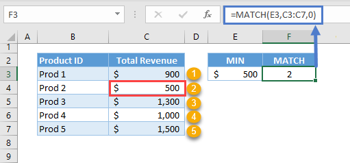
Note: We set the 3rd argument (match_type) of the MATCH Function to 0, which means exact match.
INDEX Function
The output coordinate from the MATCH Function is then fed to the INDEX Function to extract the corresponding value from the list that we are interested in (e.g., B3:B7).
=INDEX(B3:B7,F3)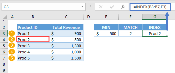
Note: If the 1st argument (i.e., array) of the INDEX Function is a 1D list, the 2nd argument (i.e., row_num) can become the row coordinate or column coordinate depending on the arrangement of the 1D list. If it’s a vertical list, then it becomes the row coordinate, and if it’s a horizontal list, then it’s the column coordinate.
Overall, the MIN Function extracts the lowest value, the MATCH Function looks up the lowest value and returns its position and the INDEX Function extracts the corresponding value from the list that we are interested. Combining all of these into one formula results to our original formula:
=INDEX(B3:B7,MATCH(MIN(C3:C7),C3:C7,0))
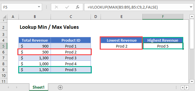
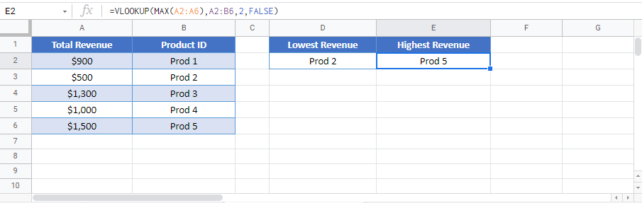
VLOOKUP with MIN
We can also use the VLOOKUP Function instead of the INDEX-MATCH Formula as the lookup formula, but we need to change the structure of our table by making the lookup column (e.g., Total Revenue) the first column.
Just like with the INDEX-MATCH, we’ll input the MIN Function as the lookup value for VLOOKUP.
=VLOOKUP(MIN(B3:B7),B3:C7,2,FALSE)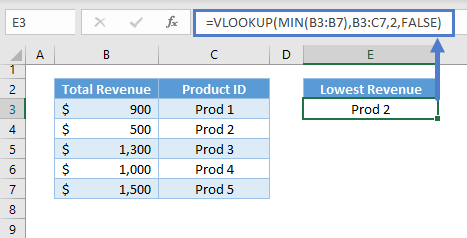
Note: The VLOOKUP Function searches for the lookup value from the first column of the table and returns the corresponding value from the column defined by the column index (i.e., 3rd argument).
XLOOKUP with MIN
Another alternative for the lookup formula is the XLOOKUP Function, which is the most convenient solution, but requires a newer version of Excel. This solution requires the fewest number of functions and there is no need to restructure data.
We can nest the MIN Function in XLOOKUP to lookup for the lowest value.
=XLOOKUP(MIN(C3:C7),C3:C7,B3:B7)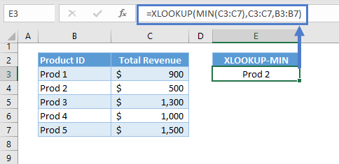
Note: By default, the XLOOKUP Function finds an exact match from the top of the lookup array (2nd argument) going down (i.e., top-down). Once it finds a match, it returns the corresponding value from the return array (3rd argument). Otherwise, it returns an error.
As discussed previously, the structure of the solutions is the same. Therefore, we’ll use one of the lookup formulas (i.e., XLOOKUP) as we move on to the succeeding sections.
XLOOKUP with SMALL
If you want to lookup the 2nd or 3rd smallest value, you can use the SMALL Function. In this example below, we’ll use the SMALL Function to extract the lowest value.
=XLOOKUP(SMALL(C3:C7,1),C3:C7,B3:B7)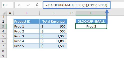
Let’s walkthrough the formula:
SMALL Function
We can return the lowest value by setting the 2nd argument of the SMALL Function to 1, which means the 1st entry if the list is in ascending order.
=SMALL(C3:C7,1)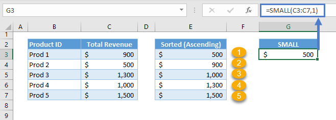
Note: instead we could use 2 for the 2nd smallest or 3 for the 3rd smallest.
Then, the result of the SMALL Function will be the lookup value to our lookup formula, which in this case is the XLOOKUP Function:

Combining the two functions results to our original formula:
=XLOOKUP(SMALL(C3:C7,1),C3:C7,B3:B7)
Lookup Highest Value
We can also find the highest value by using the opposites of MIN and SMALL: the MAX Function and LARGE Function, respectively.
XLOOKUP with MAX
We can nest the MAX Function as the lookup value for the XLOOKUP Function to lookup for the highest value.
=XLOOKUP(MAX(C3:C7),C3:C7,B3:B7)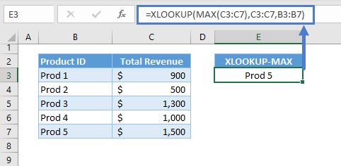
Let’s walkthrough the formula:
MAX Function
We need the MAX Function to return the largest value in the list.

The result from the MAX Function is then fed to the XLOOKUP, which will extract the value that we are interested in:
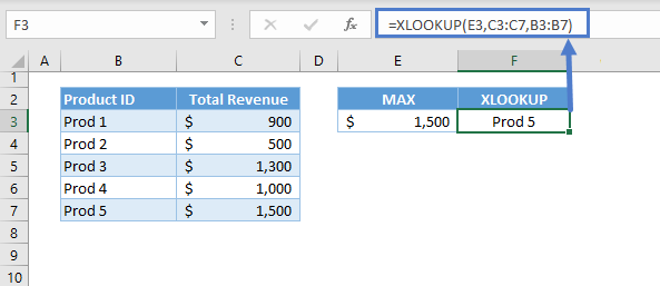
Combining the two together, we have our original formula:
=XLOOKUP(MAX(C3:C7),C3:C7,B3:B7)
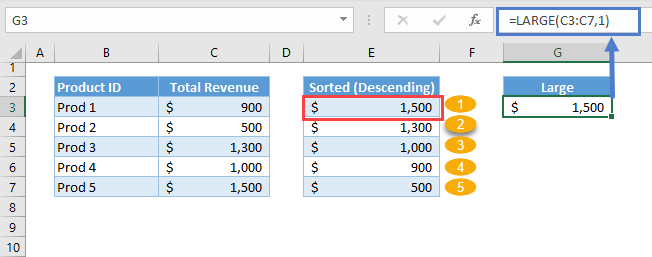
XLOOKUP with LARGE
The alternative to the MAX Function is the LARGE Function. The LARGE Function will return the nth largest number in a list. In this example we will return the largest.
=XLOOKUP(LARGE(C3:C7,1),C3:C7,B3:B7)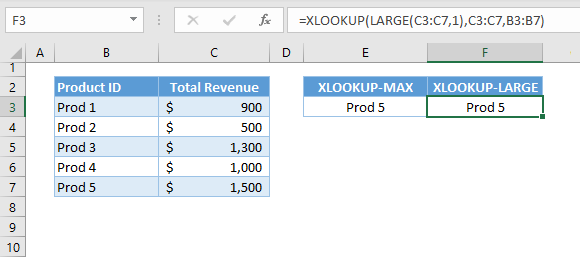
Let’s breakdown and visualize the formula:
LARGE Function
By setting the 2nd argument of the LARGE Function to 1, we can extract the largest value from the list.
The result of the LARGE Function is then used as the lookup value of the XLOOKUP:
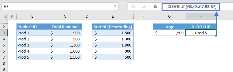
Combining the two functions results to our original formula:
=XLOOKUP(LARGE(C3:C7,1),C3:C7,B3:B7)
Lookup nth Lowest/Highest Value
XLOOKUP with SMALL nth Lowest Value
We can change the 2nd argument of the SMALL Function to greater than 1 to find the nth lowest value from the list.
=XLOOKUP(SMALL(C3:C7,2),C3:C7,B3:B7)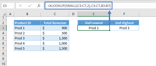
XLOOKUP with LARGE nth Largest Value
We can also do the same for the nth largest value using the LARGE Function.
=XLOOKUP(LARGE(C3:C7,2),C3:C7,B3:B7)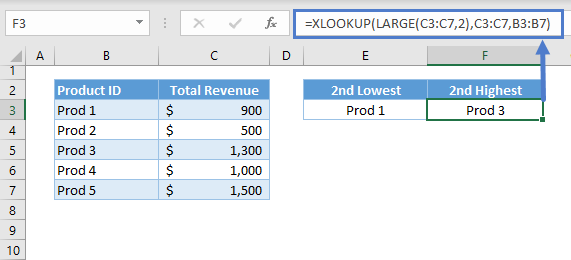
Lookup Min/Max with Conditions
In complicated scenarios where there are criteria to extract the min/max value, we can use the IF variants of the MIN and MAX: MINIFS and MAXIFS.
XLOOKUP with MINIFS
The criteria used in the MINIFS must also be applied as “AND” criteria for the lookup process.
=XLOOKUP(MINIFS(D3:D7,C3:C7,"A")&"A",D3:D7&C3:C7,B3:B7)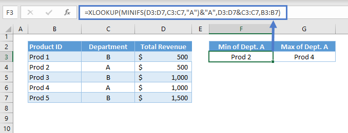
Let’s walkthrough the formula:
MINIFS Function
The MINIFS Function returns the smallest number that meets the given criteria (e.g., Department).
Note: The MINIFS Function require at least three arguments: the min_range (1st argument), the criteria_range1 (2nd argument) and criteria1 (3rd argument). The remaining arguments are optional arguments if there are more than one set of criteria_range and criteria. One important property of the MINFIS Function is that the range arguments (i.e., min_range, criteria_range) must be range of cells and can’t be array constants (e.g., {1;2;3}) or array output from other functions (e.g., SEQUENCE(3)).
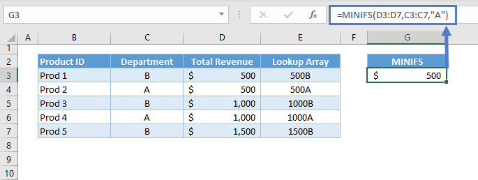
Lookup “AND” Criteria
In essence, we need to lookup the lowest value that satisfy our given criteria. This also means that our lookup process must also satisfy the criteria. Therefore, our scenario becomes a lookup with multiple criteria (e.g., Total Revenue and Department), where all of the criteria must be satisfied (i.e., AND Criteria).
The most common way to apply the AND Criteria is by concatenating the criteria using the & Operator, which stitches two values into one text. We also need to concatenate the lists where the lookup values will be searched.
=G3&"A"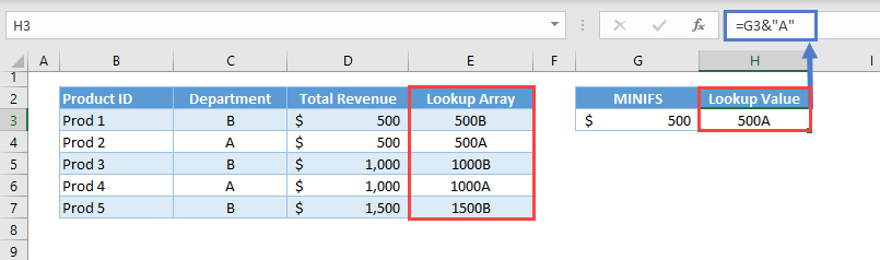
The concatenated criteria became the new lookup value (e.g., H3) and the concatenated lists became the new lookup array (e.g., E3:E7).
=XLOOKUP(H3,E3:E7,B3:B7)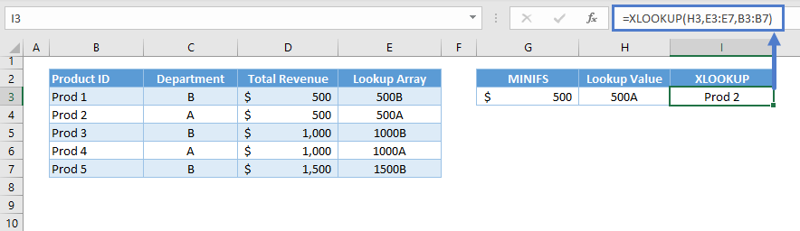
Combining all these together results to our original formula:
=XLOOKUP(MINIFS(D3:D7,C3:C7,"A")&"A",D3:D7&C3:C7,B3:B7)
XLOOKUP with MAXIFS
We also apply the same concepts from the previous section (i.e., XLOOKUP with MINIFS) for looking up the highest value that meets the given criteria.
=XLOOKUP(MAXIFS(D3:D7,C3:C7,"A")&"A",D3:D7&C3:C7,B3:B7)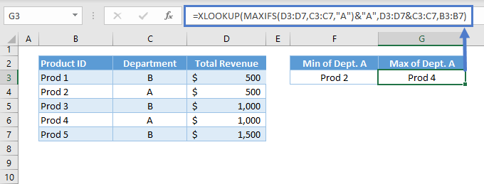
Note: The MAXIFS Function works similarly to the MINIFS Function.
Lookup Min / Max Values in Google Sheets
The formulas work the same way in Google Sheets, except the XLOOKUP Function does not exist in Google Sheets.
Get Max Value using VBA
The following function will return the Maximum Value in each Column in a Range:
Function Max_Each_Column(Data_Range As Range) As Variant
    Dim TempArray() As Double, i As Long
        If Data_Range Is Nothing Then Exit Function
        With Data_Range
        ReDim TempArray(1 To .Columns.Count)
        For i = 1 To .Columns.Count
            TempArray(i) = Application.Max(.Columns(i))
        Next
    End With
        Max_Each_Column = TempArray
End Function
We can use a subroutine like the following to display the results:
Private Sub CommandButton1_Click()
Dim Answer As Variant
Dim No_of_Cols As Integer
Dim i As Integer
No_of_Cols = Range("B5:G27").Columns.Count
ReDim Answer(No_of_Cols)
Answer = Max_Each_Column(Sheets("Sheet1").Range("B5:g27"))

For i = 1 To No_of_Cols
MsgBox Answer(i)
Next i
End Sub
So:
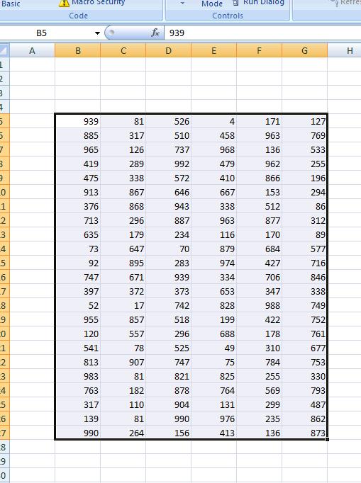
Will return 990,907, 992, 976 ,988 and 873 for each of the above columns.

