How to Create Animated Charts in Excel

This tutorial will demonstrate how to create animated charts in all versions of Excel: 2007, 2010, 2013, 2016, and 2019.

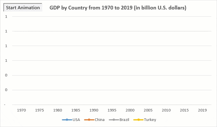
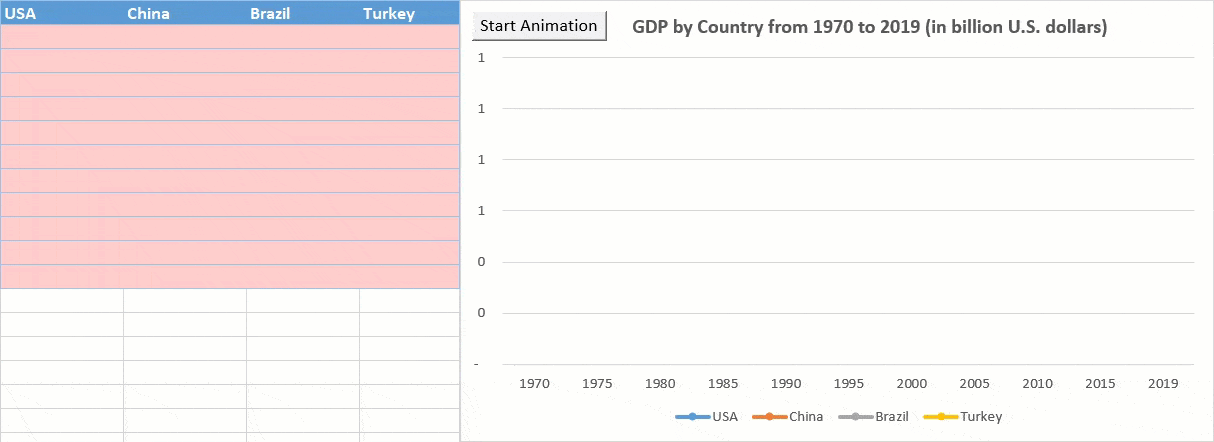
An animated Excel chart that draws itself onscreen in front of the very eyes of your audience is a powerful, attention-grabbing way to put your data in motion.

In contrast to static graphs, animated charts provide additional context to your data and helps identify emerging patterns. As an example, take a look at the animated line chart with markers shown below that demonstrates the GDP of four countries (the USA, China, Brazil, and Turkey) over the past few decades.

While the static counterpart would look like nothing special or new, the animated effect makes it possible for the chart to tell the story for you, bringing life to the motionless GDP numbers.

In this step-by-step, newbie-friendly tutorial, you will learn how to do the same thing with your data—even if you are just making your first steps in Excel.

Getting Started

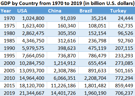
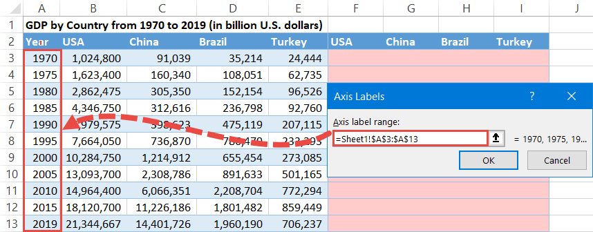
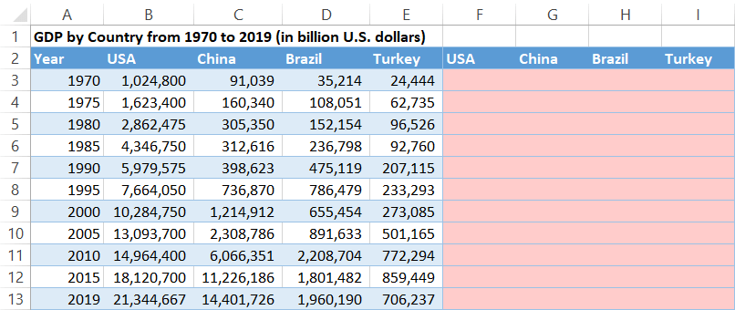
Consider the following data table containing the GDP figures for each country:

To animate the chart, we are going to use a simple VBA Macro that will smoothly plot the values on the graph.

Note: When adding VBA code to your workbook, make sure to save your workbook in .xlsm format (Microsoft Excel Macro-Enabled Worksheet) to enable macros.

Now, let’s roll up our sleeves and get down to work.

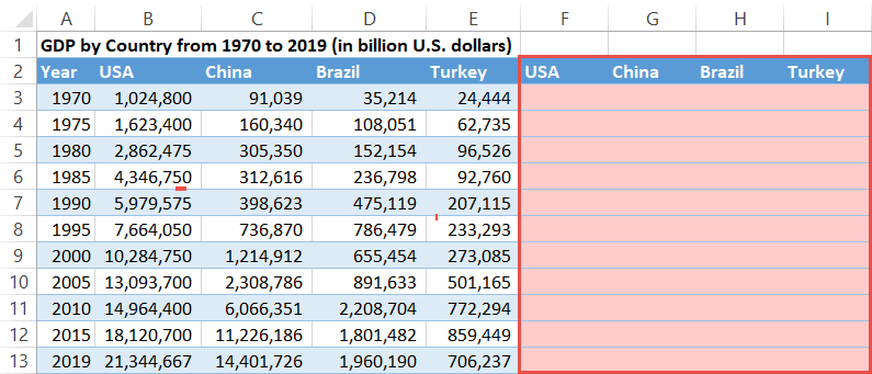
Step #1: Set up the helper columns.

To start off with, expand the data table with additional helper columns where the actual values will be gradually copied into, creating the animation effect.

Copy the headers of the columns containing the GDP numbers (B2:E2) into the corresponding cells next to the data table (F2:I2).

The cell range highlighted in light red (F3:I13) defines the place where we will store the VBA macro output.

Additionally, add decimal separators for the highlighted cell range (Home > Number > Comma Style).

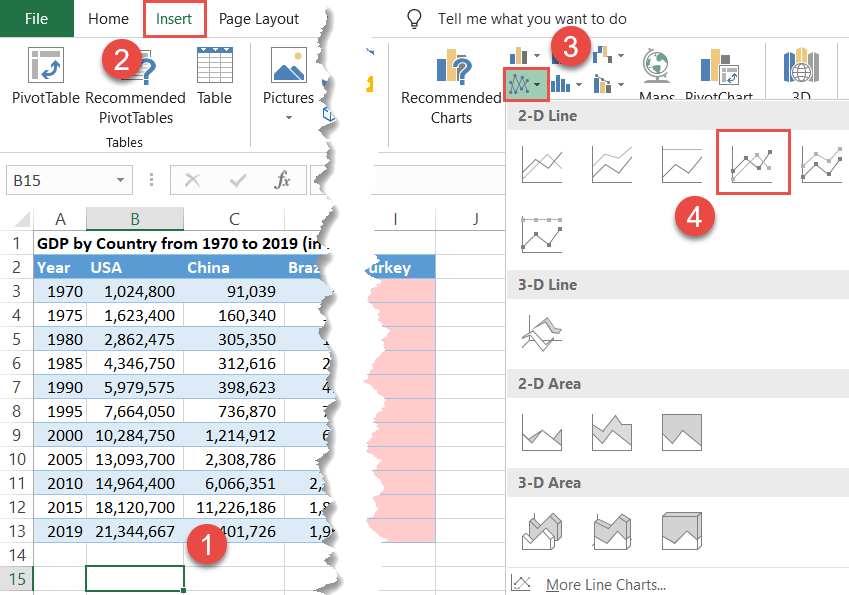
Step #2: Plot an empty chart.

Once you have allocated some space for the helper columns, build an empty 2-D chart using the columns (F2:I13) as its source data:

1. Highlight any empty cell.
2. Switch to the Insert tab.
3. Click “Insert Line or Area Chart.”
4. Choose “Line with Markers.”

Having done that, we now must link the empty chart to the cells in the helper columns (F:I). Right-click on the empty plot and click “Select Data.”

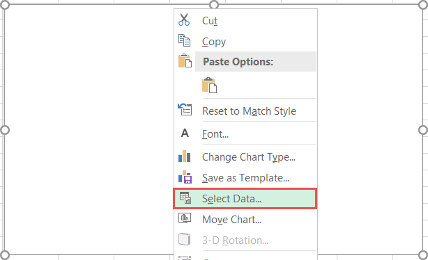
In the Select Data Source dialog box, under “Legend Entries (Series),” hit the “Add” button.

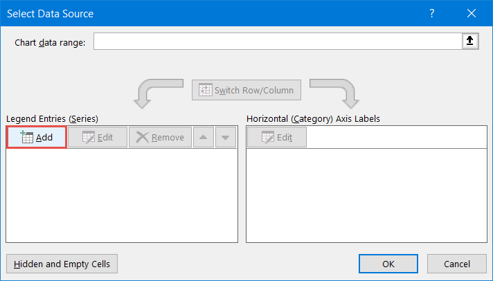
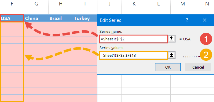
When the Edit Series dialog box springs up, create four new data series based on the helper columns (F:I):

1. For “Series name,” specify the header row cell of column USA (F2).
2. For “Series values,” select the corresponding empty cell range (F3:F13).

Repeat the same process for the remaining three columns.

Once you have your data series in place, import the horizontal axis labels to the chart.

To do that, under “Horizontal (Category) Axis Labels,” click the “Edit” button.

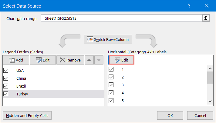
In the Axis Labels dialog box, under “Axis label range,” highlight the axis values (A3:A13).

Here’s a pro tip: If you regularly add or remove items from the data table, set up dynamic chart ranges to avoid the hassle of having to tweak the source code every time that happens.

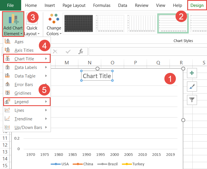
To top it off, make the future line graph even more informative by adding the chart title and legend:

1. Click the chart area.
2. Go to the Design tab.
3. Select “Add Chart Elements.”
4. Add the chart title (Chart Title > Above Chart).
5. Add the chart legend (Legend > Bottom).

Step #3: Program the VBA to create the animated effect.

Once the chart’s source data has been set up the right way, next comes the hard part—writing the VBA macro that will do all the dirty work for you in just one click.

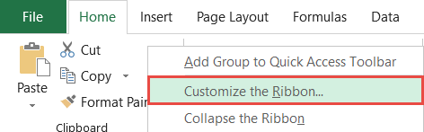
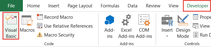
Before we dive into the nitty-gritty, make sure you have the Developer tab displayed in the Ribbon. If it is disabled, right-click on any empty space in the Ribbon and pick “Customize the Ribbon” from the menu that appears.

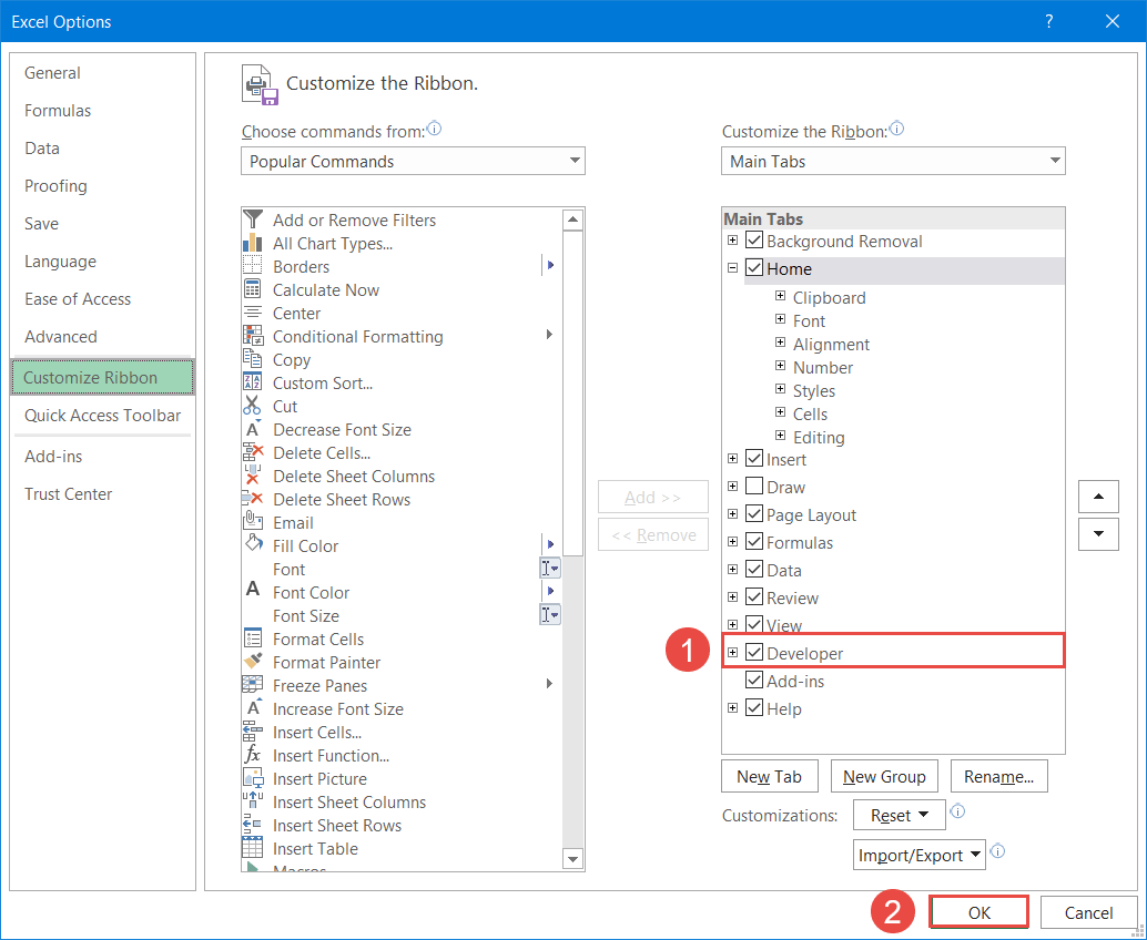
In the Excel Options dialog box, check the “Developer” box and click “OK.”

Having done that, it’s time to release the Kraken of Excel, the feature that pushes the limits of what’s possible in the world of spreadsheets. It’s time to unleash the power of the VBA.

First, open the VBA editor:

1. Navigate to the Developer tab.
2. Click the “Visual Basic” button.

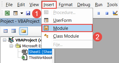
In the editor, select the Insert tab and choose “Module.”

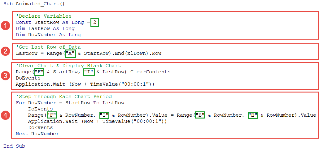
Once there, copy the following macro into the code window:

Sub Animated_Chart()

    'Declare Variables
    Const StartRow As Long = 2
    Dim LastRow As Long
    Dim RowNumber As Long

    'Get Last Row of Data
    LastRow = Range("A" & StartRow).End(xlDown).Row

    'Clear Chart & Display Blank Chart
    Range("F" & StartRow, "I" & LastRow).ClearContents
    DoEvents
    Application.Wait (Now + TimeValue("00:00:1"))

    'Step Through Each Chart Period
    For RowNumber = StartRow To LastRow
        DoEvents
        Range("F" & RowNumber, "I" & RowNumber).Value = Range("B" & RowNumber, "E" & RowNumber).Value
        Application.Wait (Now + TimeValue("00:00:1"))
        DoEvents
    Next RowNumber

End Sub

At first glance, the code may appear daunting for VBA newbies, but in reality, it takes just a few simple steps to adapt the code for your needs.

Basically, the code can be broken down into four sections as shown on the screenshot below. The green rectangles represent the segments of the code that must be tailored to your data—while the rest should remain unchanged.

Let’s zoom in on the parts you need to fine-tune. For your convenience, take another look at the data table and follow my footsteps:

Declare Variables: This section introduces new variables for the VBA to work with. In our case, the constant labeled as “StartRow” helps the VBA figure out where the data table begins (row 2). Therefore, the constant value should correspond to the row where your data starts.

Const StartRow As Long = 2

Get Last Row of Data: This line of code tells the VBA to analyze the data table and define where the data table ends (row 13) so that it can later zoom in only on the values within the specified cell range while leaving out the rest of the worksheet.

To pull it off, specify the first column (“A”) where the data table starts for the VBA to find the last row in that column that contains a non-empty cell (column A).

LastRow = Range("A" & StartRow).End(xlDown).Row

Clear Chart & Display Blank Chart: This section is responsible for erasing the values in the helper columns (F:I) each time you run the macro.

That way, you can repeat the same animated effect over and over again without having to clean up the worksheet cells on your own. To adjust, specify the first and last helper columns in your data table (“F” and “I”).

Range("F" & StartRow, "I" & LastRow).ClearContents

Step Through Each Chart Period: This is where all the magic happens. Having picked the cell range, the VBA goes row by row and fills the helper columns with the corresponding actual values at one-second intervals, effectively creating the animated effect.

To pull it off, you only need to change this line of code for the VBA to copy the values into the helper columns:

Range("F" & RowNumber, "I" & RowNumber).Value = Range("B" & RowNumber, "E" & RowNumber).Value

The first part of the code (Range(“F” & RowNumber, “I” & RowNumber).Value) grabs all the helper columns in the data table (F:I) while the second part of the equation (Range(“B” & RowNumber, “E” & RowNumber).Value) is responsible for importing the actual values into them.

With all that in mind, the “F” and “I” values characterize the first and last helper columns (columns F and I). By the same token, “B” and “E” stand for the first and last columns that contain the actual GDP numbers (columns B and E).

Once you made it through all of that, click the floppy disk icon to save the VBA code and close the editor.

Step #4: Create the macro button.

To tie together the worksheet data and the newly-created macro, set up a button for executing the VBA code.

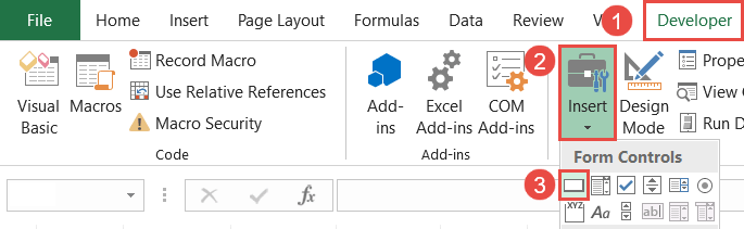
1. Go to the Developer tab.
2. Click the “Insert” button.
3. Under “Form Controls,” select “Button (Form Control).”

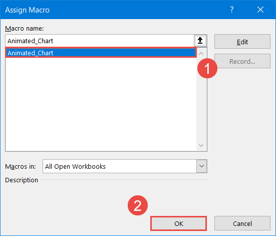
Click where you would like to place the button (preferably near the chart title). At that point, the Assign Macro dialog box will appear. Select the VBA macro you just created (Animated_Chart) and click “OK.”

As a final adjustment, change the button text (double-click button text and rename). If necessary, move the button into position where you want it.

Now, click the button and watch how the VBA smoothly fills the empty plot with the actual values—and the beauty of this method is that you can change the underlying chart type in just a few clicks without having to jump through all the hoops again!

So that’s how it’s done. Animating your Excel charts may be a great way to give a unique perspective on your data that you could have otherwise overlooked.

Obviously, it may take some time to really understand the logic behind the VBA code. But since the same code can be repeatedly reused for different types of data and charts, it’s well worth the effort to give it a try. Once you make it past the short learning curve, the world is your oyster.