SUM With a VLOOKUP Function – Excel & Google Sheets

This tutorial will demonstrate how to sum the results of multiple VLOOKUP Functions in one formula in Excel and Google Sheets.

 

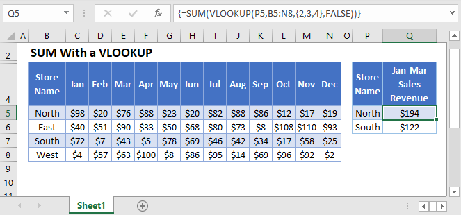
SUM with VLOOKUP

The VLOOKUP Function lookups a single value, but by creating an array formula, you can lookup and sum multiple values at once.

This example will show how to calculate the Total Sales Revenue of a specific Store over 3 months by using an array function with SUM and VLOOKUP:

=SUM(VLOOKUP(P3,B3:N6,{2,3,4},FALSE))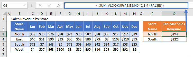

This array formula is equivalent to using the following 3 regular VLOOKUP Functions to sum revenues for the months January, February, and March.

=VLOOKUP(P3,B3:N6,2,FALSE)+VLOOKUP(P3,B3:N6,3,FALSE)+VLOOKUP(P3,B3:N6,4,FALSE)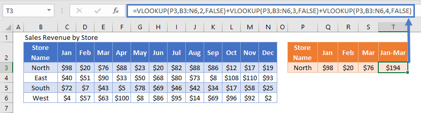

We can combine these functions together by doing the following:

First, we set the VLOOKUP Function to return columns 2, 3, and 4 as an array output (surrounding by brackets):

=VLOOKUP(P3,B3:N6,{2,3,4},FALSE)

This will produce the array result:

{98, 20, 76}

Next, to sum the array result together, we use the SUM Function.

Important! If you are using Excel versions 2019 or earlier, you must enter the formula by pressing CTRL + SHIFT + ENTER to create the Array Formula. You’ll know you’ve done this correctly, when the curly brackets appear around the formula. This is not necessary in Excel 365 (or newer versions of Excel).

Using Larger Array Sizes in a VLOOKUP Function

We can extend the size of the array input to represent more data. This next example will calculate the Total Sales Revenue of a specific Store for 12 months using an array function containing the SUM Function to combine 12 uses of the VLOOKUP Function into one cell.

{=SUM(VLOOKUP(P3,B3:N6,{2,3,4,5,6,7,8,9,10,11,12,13},FALSE))}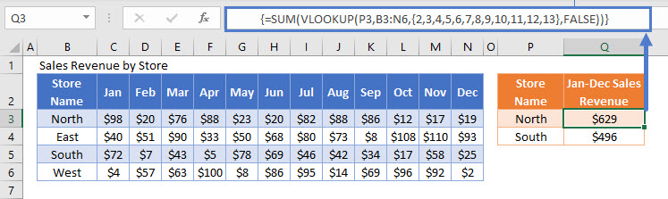

Other Summary Functions and VLOOKUP

Other summary functions can be used in the same way as the SUM Function to produce alternative summary statistics. For example, we can use the MAX, MIN, AVERAGE, MEDIAN, SUM, and COUNT Functions to summarize the Sales Revenue from January to March:

=MAX(VLOOKUP(J3,B3:H6,{2,3,4},FALSE))

=MIN(VLOOKUP(J3,B3:H6,{2,3,4},FALSE))

=AVERAGE(VLOOKUP(J3,B3:H6,{2,3,4},FALSE))

=MEDIAN(VLOOKUP(J3,B3:H6,{2,3,4},FALSE))

=SUM(VLOOKUP(J3,B3:H6,{2,3,4},FALSE))

=COUNT(VLOOKUP(J3,B3:H6,{2,3,4},FALSE))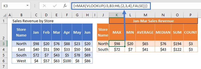

Locking Cell References

To make our formulas easier to read, we’ve shown the formulas without locked cell references:

=SUM(VLOOKUP(P3,B3:N6,{2,3,4},FALSE))

But these formulas will not work properly when copy and pasted elsewhere in your file. Instead, you should use locked cell references like this:

{=SUM(VLOOKUP(P3,$B$3:$N$6,{2,3,4},FALSE))}

Read our article on Locking Cell References to learn more.

SUM VLOOKUP Results in Google Sheets

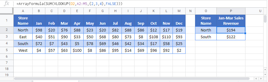
These formulas work the same in Google Sheets as in Excel, except that the ARRAYFORMULA Function is required to be used in Google Sheets for it to evaluate the results correctly. This can be automatically added by pressing the keys CTRL + SHIFT + ENTER while editing the formula.

=ArrayFormula(SUM(VLOOKUP(O2,A2:M5,{2,3,4},FALSE)))