How to Apply Cell Styles (Total, Input, Title…) in Excel

This tutorial demonstrates how to apply different cell styles in Excel.

Apply Cell Styles

Excel has some predefined cell styles to quickly add formatting. You don’t need to change cell properties one by one; just apply a style. These styles have different font sizes, backgrounds, borders, colors, etc.

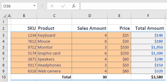
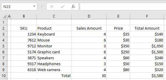
Look at the set of sales data below. It has some formatting applied (e.g., the currency number format), but applying Excel’s styles could make it easier to read.

1. First, format the table headings (B2:F2). Select the range, and then in the Ribbon, go to Home > Styles. Click the More down arrow.

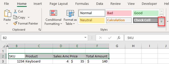
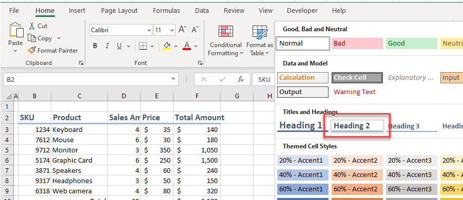
2. In the menu that pops up, choose a cell style. Here, use a style intended for headings and titles (Heading 2). As a result, cells B2:F2 are formatted as shown in the picture below.

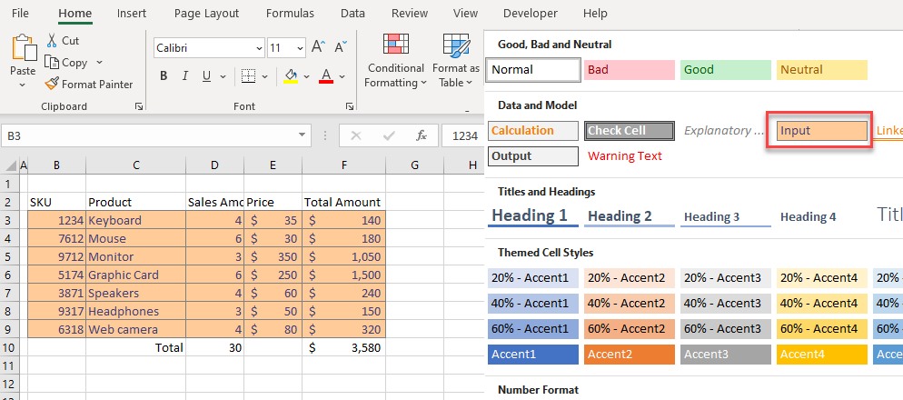
3. Next, format B3:E9 as input cells. Select the range, and then again in the Ribbon, go to Home > Styles > More.
4. Choose a cell style. Here, use a style intended for constant values: Input. As a result, cells B3:E9 are formatted as shown in the picture below.

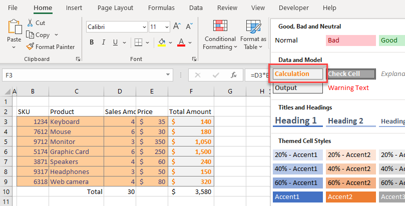
5. In the same way, format cells F3:F9 as calculation cells. Choose a cell style intended for data calculated with formulas: Calculation.

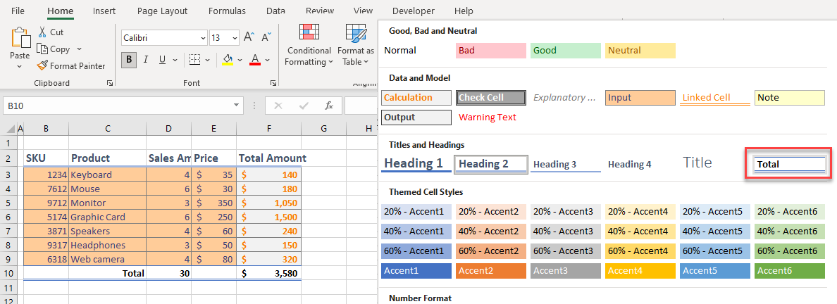
6. Finally, format cells B10:F10 as totals. Choose a cell style intended for row or column totals: Total.

Modify Cell Styles

You can also modify any of Excel’s default styles.

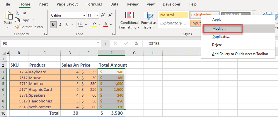
1. For example, change the font color of the Total Amounts column (cells F3:F10) to blue. Select the range.
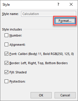
2. Then in the Ribbon, go to Home > Styles and right-click the current cell style (Calculation).
3. Click Modify…

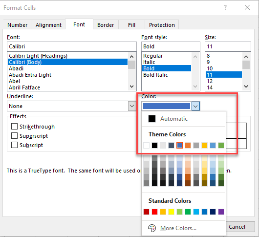
4. In the pop-up screen, click Format…

5. Go to Font > Color and choose Blue from the drop down.

The result is the style shown below, with blue font for calculation fields.

In the same way, you can change the number formats, set bold or italic, change font size, etc.