How to Create a Searchable Database in Excel & Google Sheets

This tutorial demonstrates how to create a searchable database in Excel and Google Sheets.

 

Excel has some amazing database features and is the perfect place to create a fully searchable flat-file database. A flat-file database contains all its information in a single table, with columns as the database fields and rows as the database entries. You can then use features like sorting, filters, and pivot tables.

Fields and Key Fields

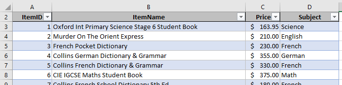
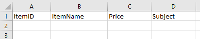
The labels you put at the top of each column describe the data that is stored in the rows beneath them. In database language, these labels are known as fields and go into the first row of the table you are creating. In the example below, these field names have gone into Row 1 of the spreadsheet.

1. Once you have created your field names, you can start entering your data. The field ItemID is a key field, used to identify a unique row of data.
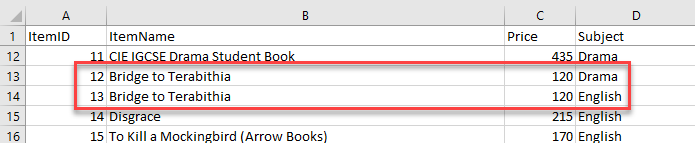
   One option is to use AutoFill to create a series of numbers, but you can use any unique identifier. For example, in the graphic below, there are two instances of a book called Bridge to Terabithia – however, they are two separate items as identified by the ItemID field.

2. If you have many rows of data, you can lock the first row of field names in place by freezing the top row of data.
   In the Ribbon, go to View > Window > Freeze Panes > Freeze Top Row.

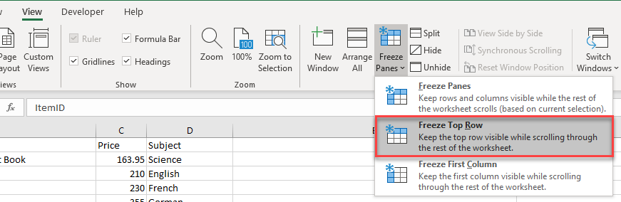
Note: If field names are not in the first row of the spreadsheet, you can still freeze the row that contains the field names. Just select the first entry in the data and click Freeze Panes instead of Freeze Top Row.

Create a Table

Once you have typed in or imported your data, you can convert the database to an Excel table and gain all of the associated benefits.

1. Click anywhere within the data, and then in the Ribbon, go to Home > Styles > Format as Table.

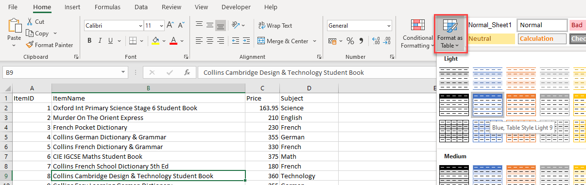
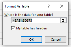
2. Choose a format to apply, and then in the Format As Table dialog box, make sure that My table has headers is checked.

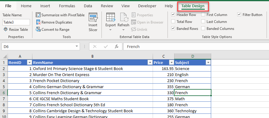
When the format is applied, a new tab called Table Design appears in the Ribbon.

Filter Data

Once you have formatted your data as a table, the ability to filter by each field is automatically applied.

1. Click on the filter button and check the value(s) you wish to filter for.

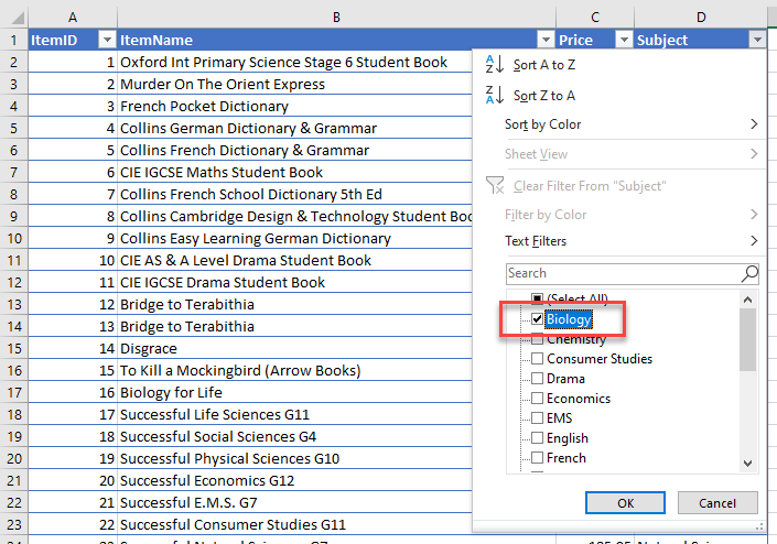
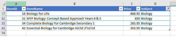
2. Click OK to apply the filter to the table, hiding all unchecked items.

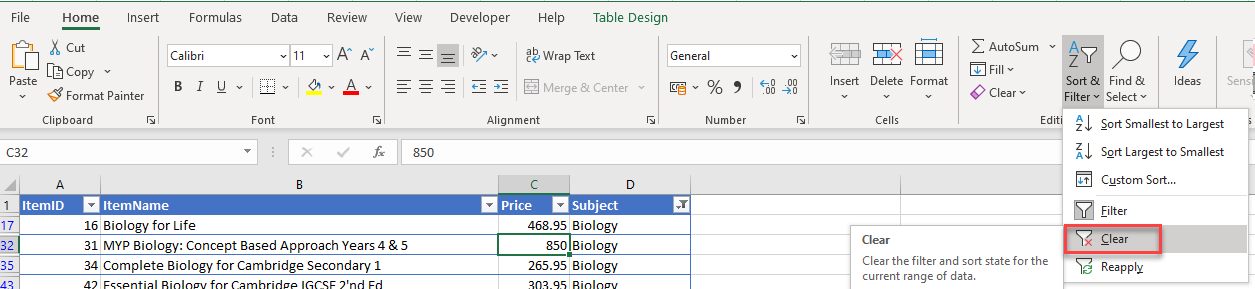
3. To clear the filter, click Select All in the filter drop down or, in the Ribbon, go to Home > Editing > Sort & Filter > Clear.

VLOOKUP Search

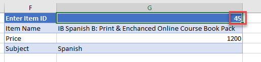
You can use the VLOOKUP Function to search for specific items in your database using the unique ID field: in this case, ItemID.

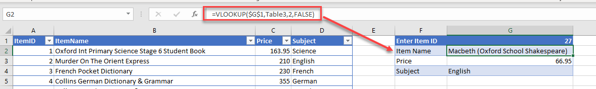
The picture below shows a vlookup table (in Columns F:G). Here, typing 45 into the search cell (G1) grabs the relevant data (in G2:G4) from ItemID #45 of the database.

Import Data

Often, you can obtain data from outside of Excel from a different data source such as a TXT, CSV, XML, or HTML file – or a different database, such as SQL or MYSQL. Import into Excel, and then clean up the data accordingly. Data comes into Excel formatted as a table.

Calculated Fields

You can add calculated fields to your database. For instance, you can combine two separate fields together or multiply fields (like quantity × price).

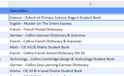
Here’s an example of a calculated field that combines two fields together.

1. Add a new field – Description – to the database shown in the example above.

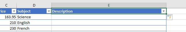
2. As soon as you type in the field name and press ENTER, the new field is added to the current table and the table is extended.
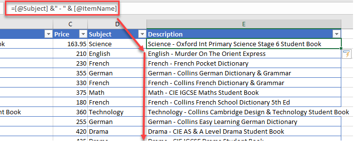
3. Then type a formula into the first row of data.

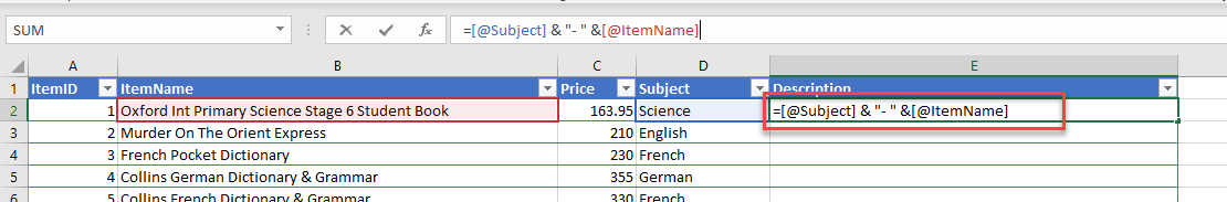
4. When you press ENTER, the rest of the table is automatically populated.

Create a Searchable Database in Google Sheets

Database functionality in Google Sheets is very similar. Once you have set up field names and typed in or imported data into your worksheet and cleaned it up, you can freeze the top row as you do in Excel.

Lock Field Names

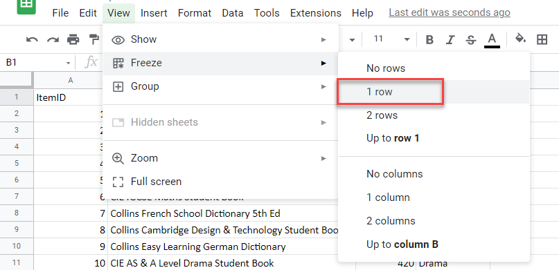
Click in the top row of your data and then, in the Menu, go to View > Freeze > 1 row.

Add Formatting

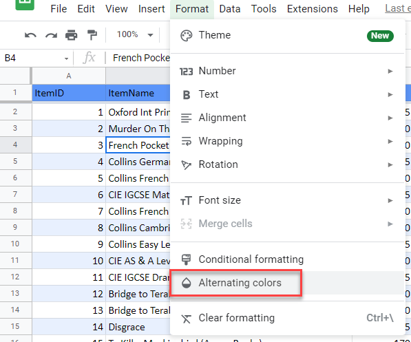
While Google Sheets does not have an option to format the data as a table, you can format the data with alternate colors to make it easier to read.

Apply Filter

You can also apply filters to the data.

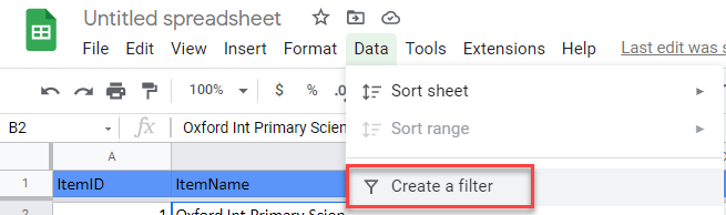
1. Select the column you wish to filter by, and then in the Menu, go to Data > Create a Filter.

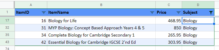
2. Click Clear to clear the checkmarks from the list and then check the item you wish to filter for (here, Biology).

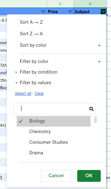
3. Click OK to filter the data, hiding all unchecked items.

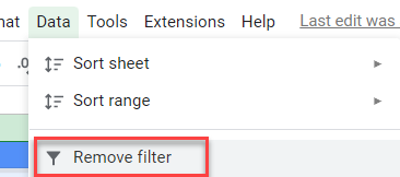
4. To clear the filter, click Clear in the filter drop down. Or in the Menu, go to Data > Remove filter.

Insert New Fields

1. To add a new field to the database, type the field name in the next available column to the right of the data.

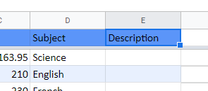
2. As soon as you press ENTER, the field is added to the table and formatted accordingly.
   You can now create a calculated field as you did in Excel.

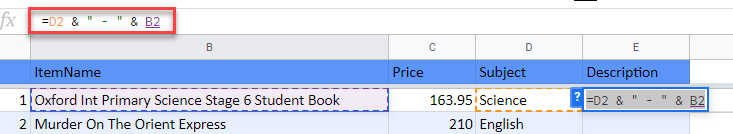
3. When you press ENTER, you get the option to autofill the database.

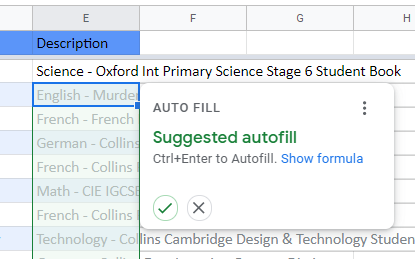
4. Click the checkmark to copy the formula down.