How to Cross-Reference in Excel & Google Sheets

This tutorial demonstrates how to cross-reference other data in Excel and Google Sheets.

 

An Excel workbook can be made up of multiple worksheets. There’s often a benefit to cross-referencing cells from one sheet to another (or even just two locations on the same sheet). For example, you might be creating a summary worksheet that refers to other worksheets in your file. You can do this by creating formulas that refer to or cross-reference the other sheets. You can also create formulas that refer to or cross-reference other Excel files (workbooks). That way, there’s no typing and retyping the same values, and changes are easier to make across the workbook.

The worksheet supplying the data is called the source worksheet while the worksheet containing the reference is termed the dependent worksheet.

Reference Another Sheet With Paste Special

1. 1. Select the cells in the source worksheet you wish to link to the destination sheet, and then in the Ribbon, go to Home > Clipboard > Copy, or press CTRL + C on the keyboard.

2. In the destination sheet, select the cells where you wish to insert the linked data.

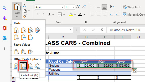
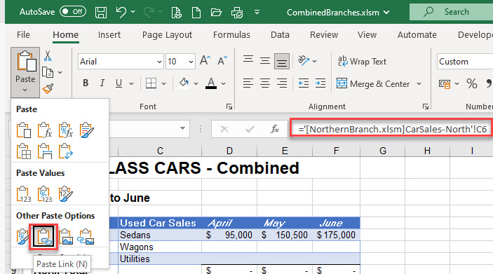
3. In the Ribbon, go to Home > Clipboard > Paste > Other paste Options > Paste Link.

Paste Special Dialog Box

Instead of Steps 1–3 above, you can use this alternate Paste Special method.

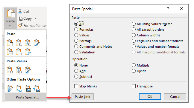
1. In the Ribbon, go to Home > Clipboard > Paste > Paste Special, and then click Paste Link.
   Tip: The shortcut to open the Paste Special dialog box is CTRL + ALT + V.

2. Linked formulas are created for you linking the destination cell references to the source cell references.

Reference Another Sheet Manually

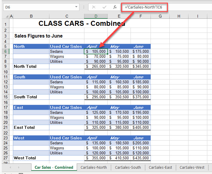
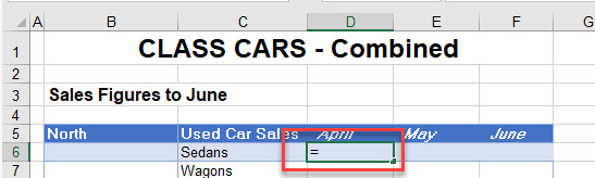
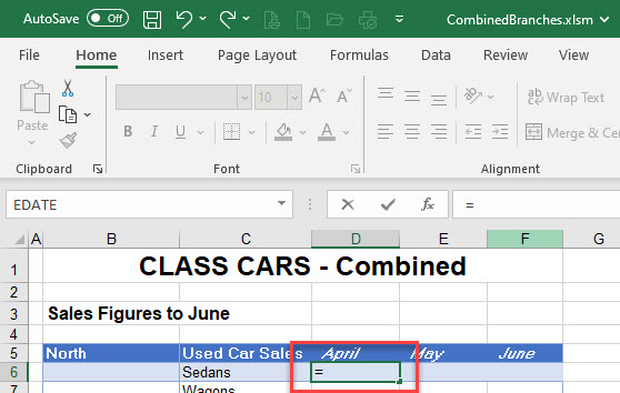
1. Click in the cell in your destination sheet where you wish the linked formula to be placed, and then type equals (=) on the keyboard to begin your formula.

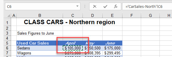
2. Select the source sheet (the sheet the value is coming from), and then click on the source cell.

3. Press ENTER to complete your formula.

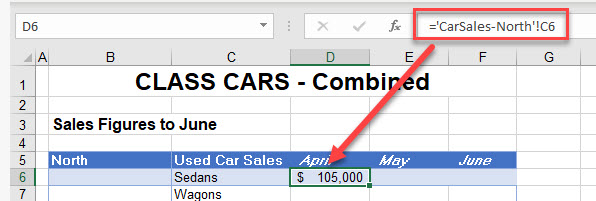
4. When a linked formula is created between two sheets (either by Paste Special or manually) the syntax of the linked formula is always:

='Worksheet'!CellReference

5. 5. If the sheet name contains spaces or any characters that are not alphanumeric (such as a hyphen, in this case), it is contained between single quotation marks. It always have an exclamation mark after it, and then the cell reference follows to complete the formula.

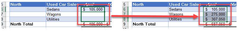
=CarSales-North!B6

6. Once you have created a linked formula, you can copy the formula down and across, as long as the formula does not contain any absolute (anchored) references.

Create a Linked Formula With Range Name

If you don’t usually work with named ranges, jump to Learn About Range Names below for some background.

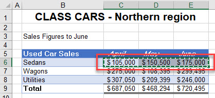
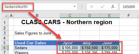
1. If you have range names in your source worksheet, you can create linked formulas to these range names.
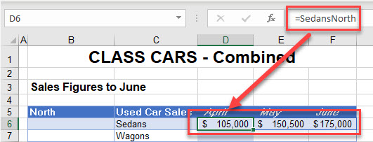
2. The worksheet shown below has a range name called Sedans-North, which refers to cells B6:D6.

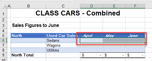
3. In the destination worksheet, click in the cell where you need the formula to go and type the equal sign (=).

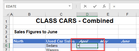
4. Switch to the worksheet that contains the range name you want, and then select the named range.

5. Press ENTER to complete your formula. Notice that the cells adjacent to the cell where you entered the equal sign are also populated with the correct formula.

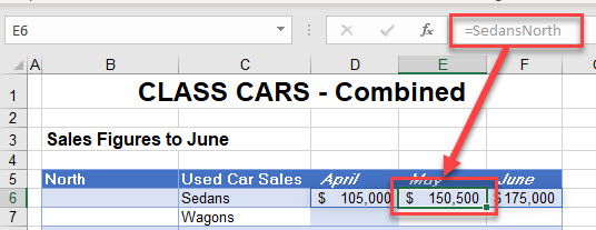
6. However, if you click on one of the adjacent cells, you can see that the formula is grayed out. This is because an array formula has been created. In older versions of Excel, you had to press CTRL + ENTER on the keyboard but the IntelliSense in the newer versions of Excel do this for you. You cannot, however, delete a formula unless you are on the original cell where the formula was created (in this case, C6).

Learn About Range Names

Basics

• What and Where are the Name Manager and Name Box?
• How to Use the Name Box
• How to Create Range Names from Selection
• How to Edit Named Ranges
• Find the Location of a Named Range
• How to Delete Named Range(s)

Shortcuts

• Open Name Manager Dialog Box
• Insert Named Range Into Formula
• Create Name Based on Row and Column Headings

More

• Dynamic Named Range Based on Cell
• How to Fix the #NAME? Error
• How to Resolve a Name Conflict for a Named Range
• How to Paste Range Names
• How to Rename a Table

Reference Another File With Paste Special

1. You can also link two separate Excel files (workbooks) together using linked formulas.
2. Before you link two files together, make sure that both files are open and have been saved with any recent changes.

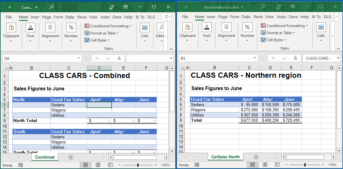
3. As with linking two worksheets together, in the source workbook, select the cell references to copy, and then in the Ribbon, go to Home > Clipboard > Copy, or press CTRL + C on the keyboard.

4. Click back in the destination workbook and select the cell references where you wish the linked data to go.
5. In the Ribbon, go to Home > Clipboard > Paste > Other paste Options > Paste Link.

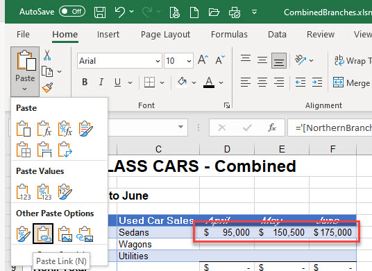
6. A linked formula is created in each of the selected cells. This formula differs slightly from when you are linking worksheets in the same file; this external link formula contains the name of the file as well as the name of the sheet.

Reference Another File Manually

1. As with creating a formula between two worksheets, you can manually create a formula between two open files (workbooks).
2. Select the cell in your destination workbook where you wish the linked formula to be placed, and then type equals (=) on the keyboard to begin your formula.

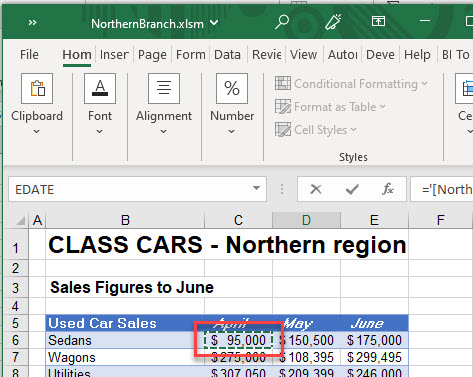
3. Select the source workbook and the sheet the value is coming from and click on the source cell.

4. Press ENTER to complete your formula.

5. When a linked formula is created between two files (either by Paste Special or manually) the syntax of the linked formula is:

='[FileName] WorksheetName'!Reference

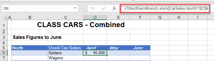
6. 6. The name of the workbook is enclosed in square brackets while the file name and the worksheet name is contained between single quotation marks. An exclamation mark follows, with the cell reference following to complete the formula. For example:

='[NorthernBranch.xlsm]CarSales-North'!B6

7. 7. 7. Notice that, when a formula is created manually between two files (as opposed to using Paste Link), the cell references in the formula are automatically put in as absolute (or anchored) references. You can’t copy the formula across or down unless you change your formula to remove the absolute (dollar) signs.

Tip: Use the shortcut F4 to cycle through relative/absolute references in formulas.

Cross-Reference in Google Sheets

You can link between two sheets in a Google Sheets file by manually creating a formula between them.

1. In the destination file, select the cell where you want the formula to go, and then type equals (=).

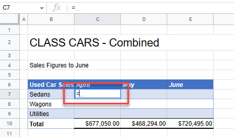
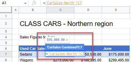
2. Go to the source sheet and select the cell you want.

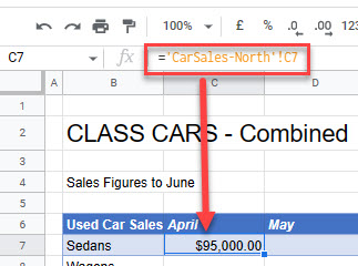
3. Press ENTER to complete the formula.

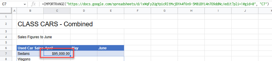
4. It is possible to link two separate Google Sheets files together using the IMPORTRANGE Function (unique to Google Sheets).
5. Make sure both the destination and source files are open, and then copy the URL of the source file.

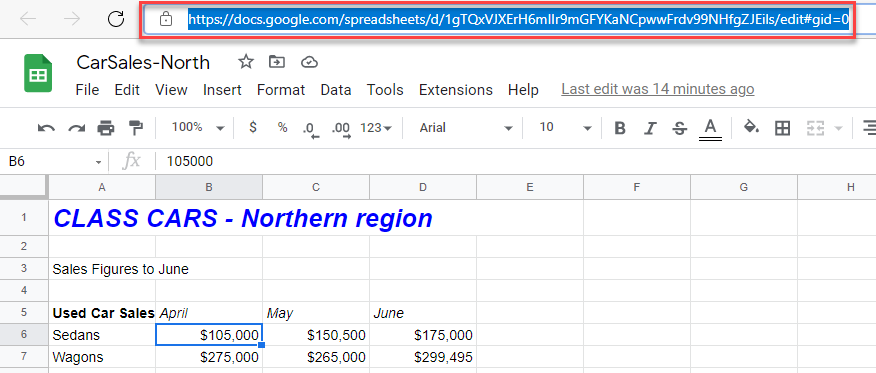
6. Switch back to the destination file, and in the cell where you want the link to go, enter the following formula:

=IMPORTRANGE("https://docs.google.com/spreadsheets/d/1xWqFy2UgYpicRItMvjBYA4f6n9-5M8iBYi4n7O9ddNc/edit?pli=1#gid=0", "C7")

7. You may need to give your file access to the source file.

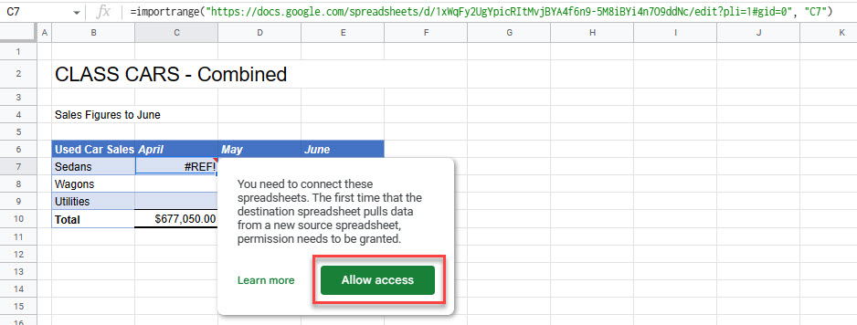
8. Click Allow access to complete the formula.