6 Tips to Clean Up Data in Excel & Google Sheets

This tutorial demonstrates how to clean up data in Excel and Google Sheets.

Excel is, for all intents and purposes, a flat-file database; it holds data organized logically into rows and columns. Good, clean data is essential in most of the functionality you need from Excel. There are often issues, however, with data that can cause numerous problems such as extra spaces, blank rows or columns, spelling mistakes, or numbers stored as text.

This tutorial lists and walks through common issues with imported data and how to address them, cleaning up the data and making it suitable for use with Excel’s commands, features, and formulas. This list, though not exhaustive, will help in identifying issues for cleanup.

1. Take care in how you fill in the sheet to start with.
2. Fix columns. Check that there’s a column for each field and that it contains the correct data. Concatenate any columns that were unintentionally split, and delete any empty columns.
3. Check for formula and value errors and run a spell check.
4. Get rid of issues like blanks, duplicates, and trailing spaces.
5. Replace incompatible characters.
6. Format the data to make it more readable and engaging.

Similar considerations go into ensuring clean data in Google Sheets. Click here to jump to the Google Sheets section.

1. Get Data

Enter Clean Data

In some instances, you’ll be entering data directly into Excel, and you can check for accuracy as you go. See How to Create a Searchable Database for tips and instructions.

Import Data Into Excel

However, you can also import large amounts of data from external sources such as TXT files or CSV files. This is a convenient and versatile capability of Excel, but imported data can often have errors that must be removed or repaired to ensure the imported data set is accurate and aligns with your needs. Or it might need to be altered and used differently from when it was originally set up.

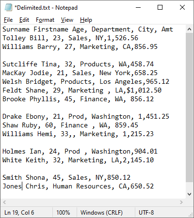
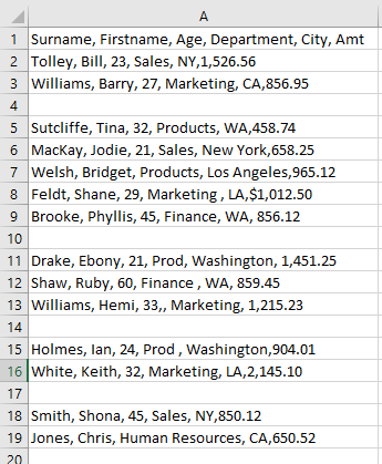
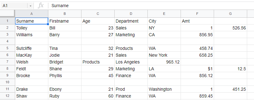
Say you have a text file like the one below.

At first glance, the data looks good, so you import it into Excel using Get Data (Power Query).

1. In the Ribbon, go to Data > From Text / CSV and choose the file (here, Delimited.txt).

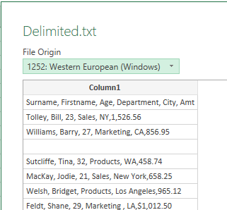
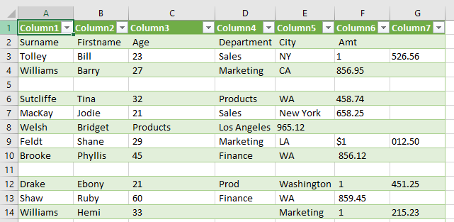
2. Because it is a TXT file, it all imports into a single column. Use the Text to Columns Wizard to separate the comma-delimited data into columns.

The imported data comes in formatted as a table, but it’s not a table you can use yet, so remove all formatting.

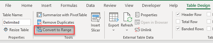
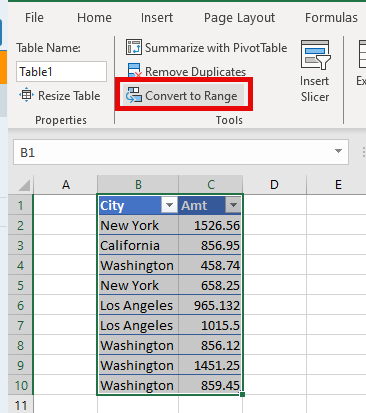
3. First, convert the table to a range. Click anywhere in the table, and then in the Ribbon, go to Table Design > Tools > Convert to Range.

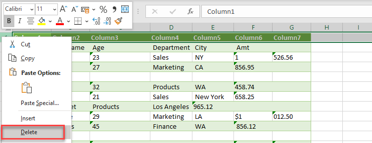
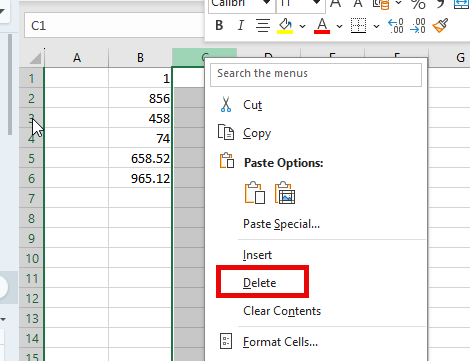
4. There were headers in the text file that weren’t picked up as headers, and an irrelevant top row was added. To remove that top row, select it, and then right-click > Delete.

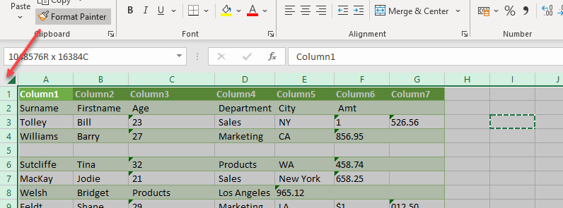
5. Finally, to remove the rest of the formatting, select an unformatted blank cell in the worksheet and then, in the Ribbon, go to Home > Clipboard > Format Painter.

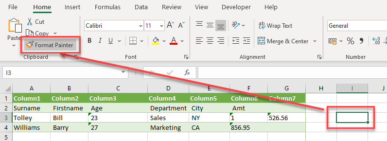
6. Then click in the Select All box at the intersection of the row and column headers.

More About Importing Data

• Convert a CSV File to XLSX
• Convert a Spreadsheet to a Delimited Text File
• Import a Word Document
• Import an HTML Table
• Open a Text (.txt) File
• What is the Difference Between CSV Files and Excel Files?

2. One Field per Column

Move Data to Correct Columns

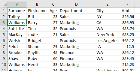
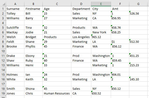
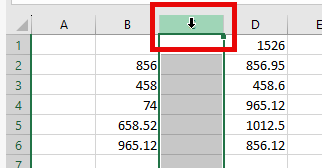
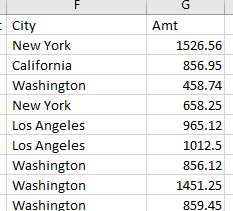
Data may come in but end up in incorrect columns, such as in Row 19 above where the data in Column C should be in Column D. Much of the time it requires manual cleaning – actually moving the data from Column C to Column D. On other occasions it may require splitting data where all the data has come in to one column when it should have been separated.

Combine Two Columns

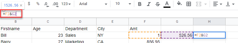
If a column has been split in error, for example, because the cell contains a comma, combine those two (or more) columns.

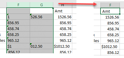
1. In the data imported above, the amount field contained a comma when the number was greater than a thousand. You can use a formula with an ampersand to combine these figures.

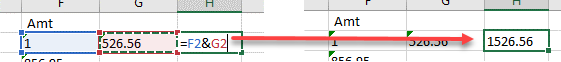
2. As this is now a calculated field, you can copy it down to the rest of the data.

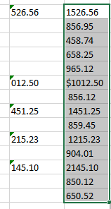
3. You can then copy and paste values to change the data from a calculated field back into text.

4. Now, move the heading (Amt) to the new column and delete the two columns to the left of it.

Remove Blank Columns

If imported data has some blank columns, you can remove them.

1. Select the blank column by clicking on the column header.

2. Right-click and Delete.

3. Correct Errors

Error Checking Command

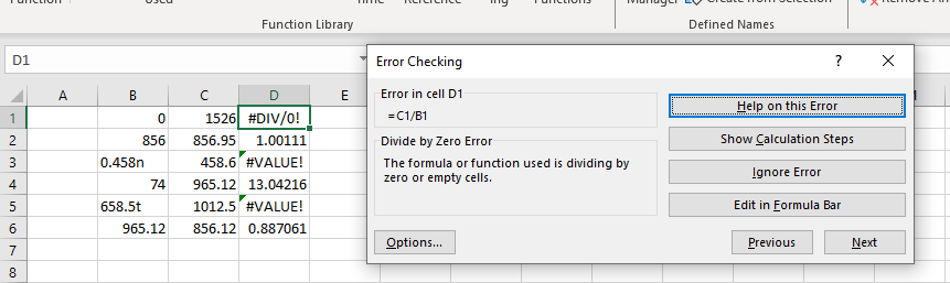
You can use the Error Checking command to check for invalid data in Excel. If you have a formula that is not calculating, it may show as #DIV/0! or #VALUE.

1. To check for these errors, in the Ribbon, go to Formula > Formula Auditing > Error Checking.

2. The Error Checking window pops up. If your data contains errors, it contains information about the first error that it encountered.

3. If you click in your data to fix the error, you can then click resume to continue with the error checking.

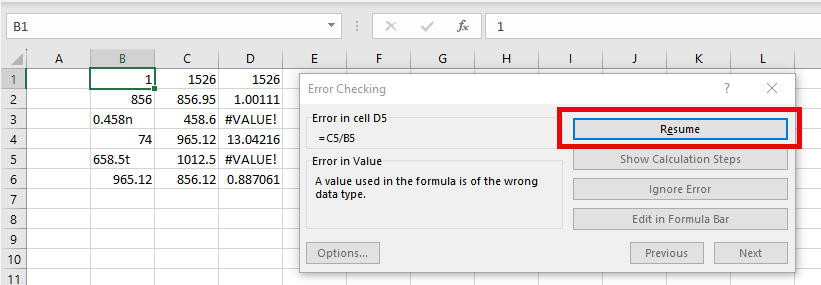
4. You can click Next to move through the errors in your data and deal with them as you see fit (ignore it, edit it, or show the calculation steps). Once you have dealt with all the errors, you see a message box.

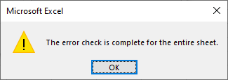
5. Click OK to end the error check.

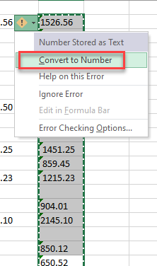
Change Text to Numbers

Numbers brought in as text need to be converted to numbers in order to be used in calculations.

To convert text to numbers, highlight the cells containing this error, click the yellow exclamation mark icon, and choose Convert to Number.

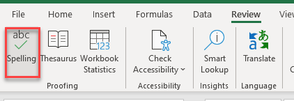
Spell Check

Spelling mistakes can easily come into Excel with imported data. A good idea is to spell check the data once it is imported.

1. In the Ribbon, go to Review > Proofing > Spelling.

2. Choose the correct word from Suggestions, and then click Change.

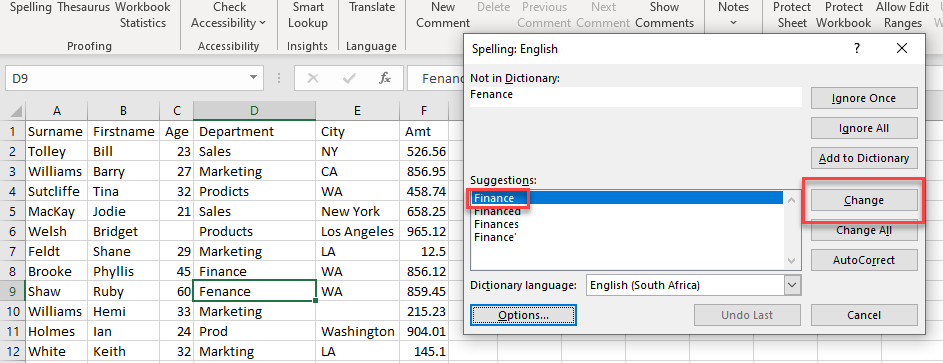
3. Ignore a word if the spelling is correct but not recognized by Excel. You can add any words like this to the Dictionary so that they do not come up as spelling errors in future.

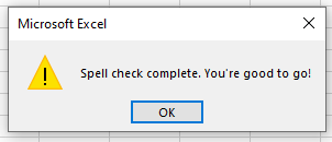
You get the message pictured below when the spell check is finished.

4. Get Rid of Extraneous Data and Cells

Remove Blank Rows

Blank rows are a nightmare in Excel data. You can manually delete the blank rows by selecting the first blank row, and then in the Ribbon, go to Home > Cells > Delete Sheet Rows.

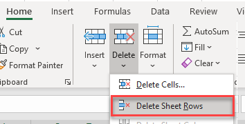
This deletes the selected row. Select the next row, and then press F4 on the keyboard. F4 in Excel repeats your last action and is an efficient way to go down and delete the rows you don’t need.

Alternatively, to delete blank rows from the data all at once, follow the instructions here.

More About Keeping Columns and Rows Consistent

• Copy Column Widths
• Copy Row Height
• Unmerge Cells
• Filter Merged Cells
• Make All Rows and Columns the Same Height and Width
• Resize Multiple Rows or Columns at Once
• Resize Cells to Default Row Height

Remove Duplicate Rows

You may find that data has been imported into your file that has some rows that are identical to other rows. In these instances, you can Remove Duplicate Rows.

1. Click in your data, and then in the Ribbon, go to Data > Data Tools > Remove Duplicates.

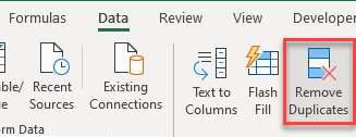
2. This selects the entire dataset. Choose which columns to check for duplicates. To check for duplicate rows, leave all columns ticked.

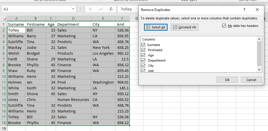
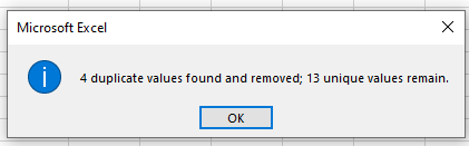
3. Click OK to remove the duplicate rows.

More About Duplicates

• Clear Duplicate Cells
• Merge Lists Without Duplicates
• Remove Unique Values
• Filter Duplicate Values
• Removing Duplicate Values in Excel with VBA

AutoMacro | Excel Automation Made Easy | Free Trial

Remove Trailing Spaces

You may find that data coming in from external sources (especially from external databases) has trailing spaces contained within the cell. While these may not seem to be a huge problem, they can affect sorting or calculations.

Remove any trailing spaces with the TRIM Function.

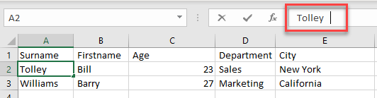
1. Insert a new column to the right of the data.
2. In the adjacent blank cell, type in the formula:

   =TRIM(A2)

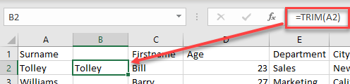
3. Copy the formula down to the rest of the data.

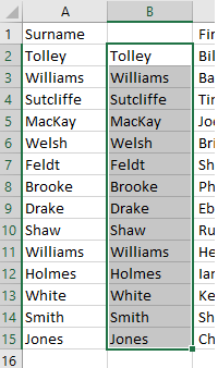
4. Copy and paste the data back as values.

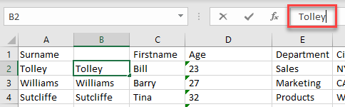
5. Move the heading (Surname) to cell B1 and delete Column A.

5. Find and Replace Text

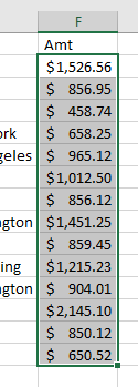
1. Use Find and Replace to remove characters you do not need.For example, a dollar sign can prevent a value from being recognized as Excel as a number.

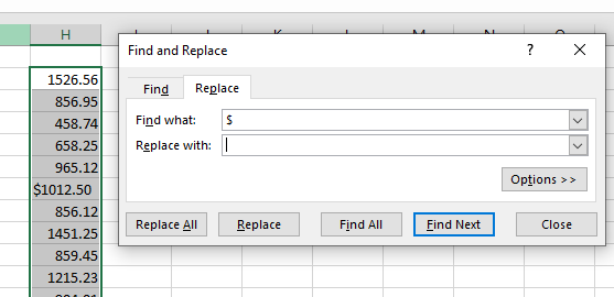
2. Then, to show the dollar sign again while making sure the values are picked up properly, format the column with the currency format.
   In the Ribbon, go to Home > Number and click Currency.

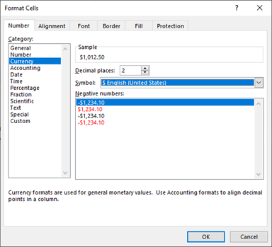
3. Click OK to apply the currency you chose to the selected data.

4. You can also use Find and Replace to replace inconsistent text and make fields ready for analysis.

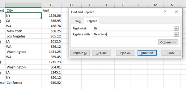
5. Repeat as often as necessary.

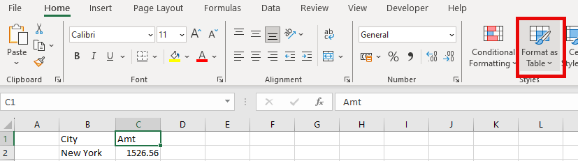
6. Format Cells

Once the data is in good shape, you’ll probably want to add formatting so it’s easier to read. One of the easiest ways to format cells is to use the Format as Table command.

1. Click in your data, and then, in the Ribbon, go to Home > Styles > Format as a Table.

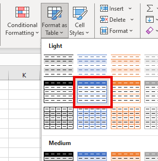
2. Choose a style from the drop down.

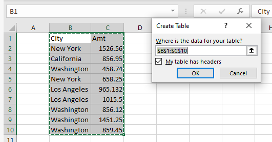
3. Make sure that the range selected is correct, and that (if necessary) the checkbox My table has headers is ticked, and then click OK.

4. Your data is automatically put into a table and formatted according to that table style. If you do not want to use your data in a table, or use the Excel table functions (of which there are many), you can covert the table back to a normal range by using the Convert to Range command in the Ribbon.

Our How To page has plenty of tutorials for applying formatting. Here are a few you may find helpful:

• Limit Decimal Places
• Hide Overflow Text in a Cell
• Add Units to Numbers
• Stop Changing Numbers to Dates
• Apply and Change Themes
• Make Cells Bigger to Fit Text
• Automatic Formatting

Clean Up Data in Google Sheets

AutoMacro | Excel Automation Made Easy | Free Trial

Import Data Into Google Sheets

You can import data into Google Sheets like you do into Excel.

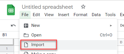
1. Open a new sheet and in the Menu, go to File > Import.

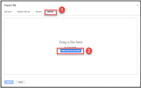
2. Click Upload, then Select a file from your device.

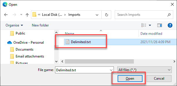
3. Choose the file you wish to import, and then click Open.

4. Change the Import location and Separator type, and then click Import data.

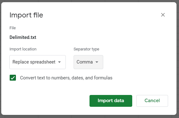
Now you have a Google spreadsheet populated with the data from your file.

Clean Up Imported Data

Cleaning up data in Google Sheets is a lot like cleaning up data in Excel.

1. Move data imported into the wrong column manually by selecting the data and dragging it across to the correct column.

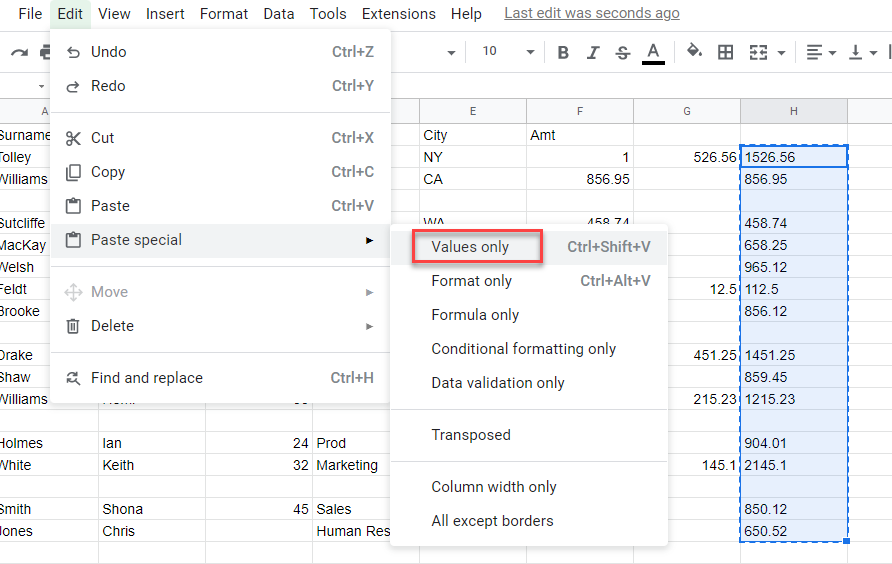
2. As in Excel, you can use a formula to combine columns as needed.

3. Drag the formula down, then use Paste Special to replace the formulas with values.

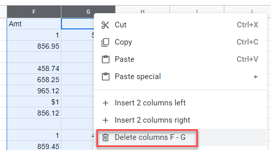
4. Then select the two original columns (in this case, Columns F and G), and right-click on the column header to delete.

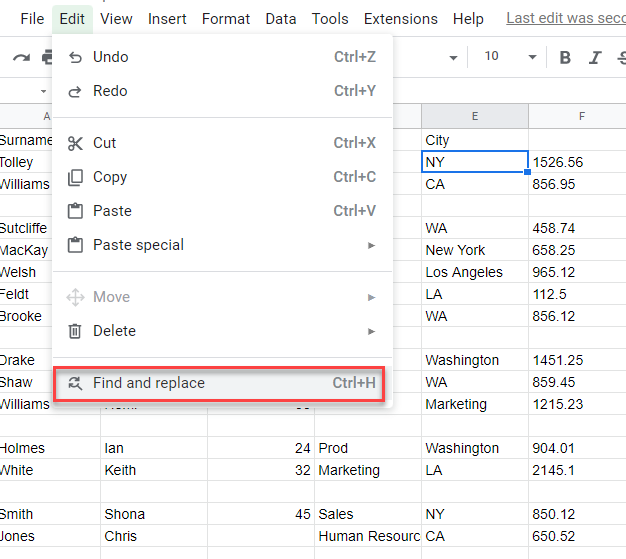
5. Use Find and Replace to remove extraneous characters, make entries consistent, etc.
   In the Menu, go to Edit > Find and replace.

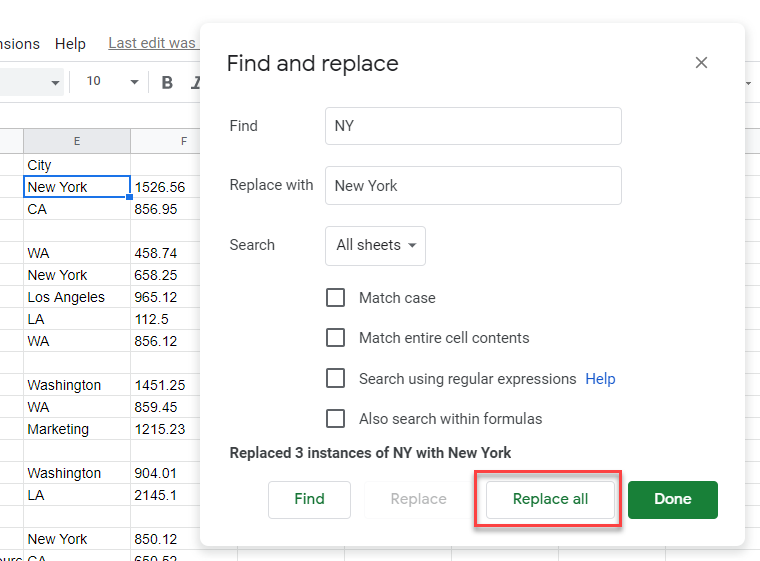
6. Type in the text you want to find and the text you want to replace it with. Then click Replace all.
7. Repeat as often as necessary. Click Done to exit Find and Replace.

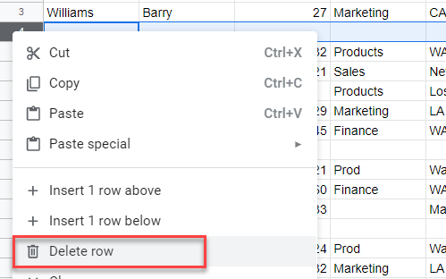
8. To remove a single blank row in the data, right-click on the row header and click Delete row.

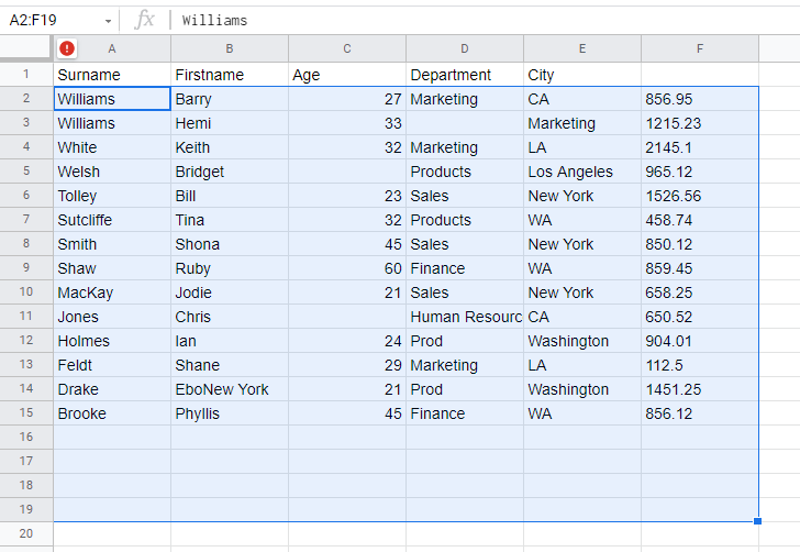
9. To remove all blank rows in the data, select the data, and then in the Menu, go to Data > Sort range > Sort range by column A (Z to A).
   When you select the data to sort, make sure to exclude column headers from your selection.

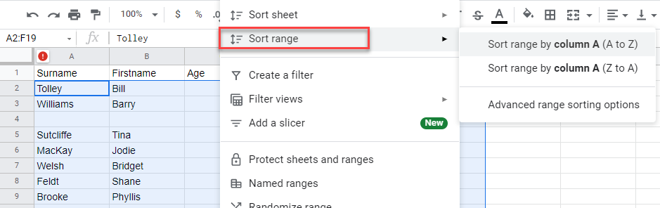
This moves all the blank rows to the bottom of the data, in effect removing them from the data.

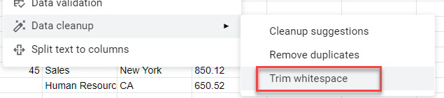
10. To remove trailing spaces from the data, go to Data > Data cleanup > Trim whitespace.

Google’s Smart Cleanup Feature

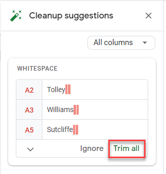
Optionally, before you start cleaning the data, you can ask Google for cleanup suggestions.

1. In the Menu, go to Data > Data cleanup > Cleanup suggestions.

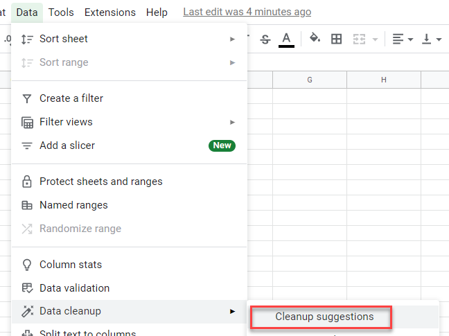
2. If Google has any cleanup suggestions, they appear in the right-hand task pane in your Google sheet.
   In the example below, it has found whitespaces at the end of some words. Click Trim all to remove the spaces.

You could also use this feature once you have completed cleaning the data to check for anything you may have missed. Don’t let this be your only check, though! It’s still important to review the data with your specific needs in mind.