How to Filter Rows in Excel & Google Sheets
Written by
Reviewed by
This tutorial demonstrates how to filter rows in Excel and Google Sheets.
Excel enables you to store data in a table format made up of rows and columns. These tables are often in database format with the columns as the headers (database fields), and the rows as the database entries. Excel then has some fabulous database features, one of which is the ability to filter data. Filtering data enables you to locate and report on a subset of the data.
In this Article
AutoFilter
AutoFilter applies drop-down filter buttons to each column of your data in Excel at once, allowing you to find, show, and hide values in one or more columns of data. You can filter based on choices supplied in a list, or you can customize the text or values to filter for.
Create an AutoFilter
▸ Click within the data range, and then in the Ribbon, go to Home > Editing > Filter.
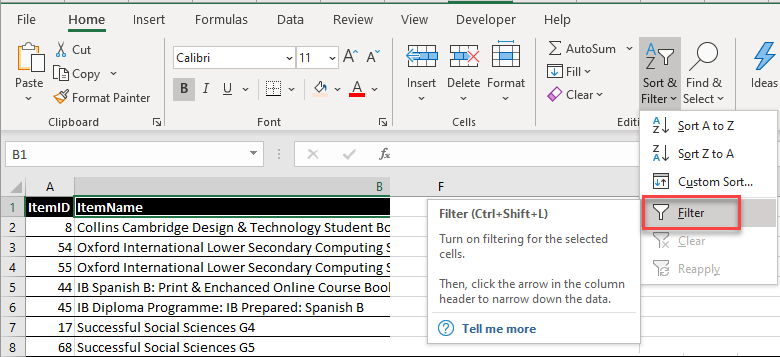
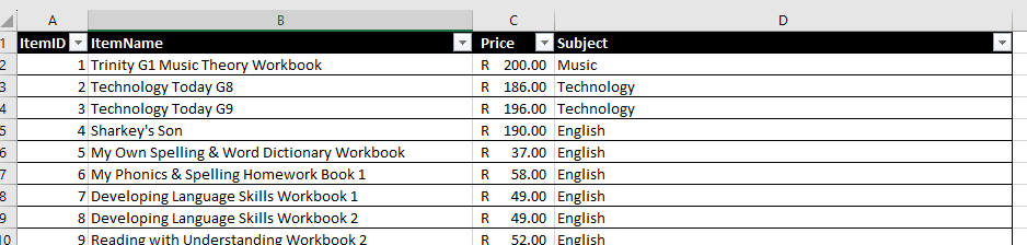
Small drop-down arrows (filter buttons) are applied to the header row of your data. Click on one of the arrows to start filtering your data.
Tip: The shortcut to apply an AutoFilter is CTRL + SHIFT + L.
Filter Text
- Click on the arrow to the right of the heading you wish to filter on, and then remove the checkmark from Select All.
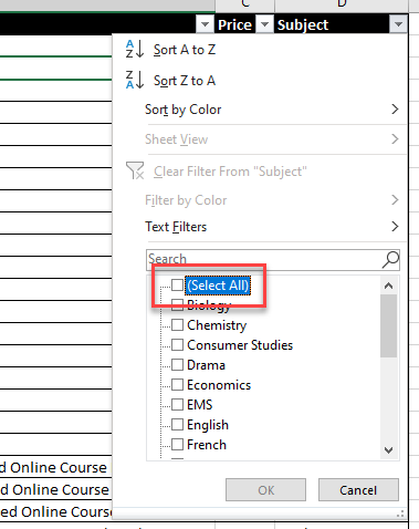
- In the list of entries shown, tick each one you want to display in the filtered data.
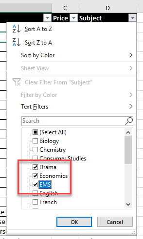
- Click OK to show the data.
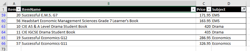
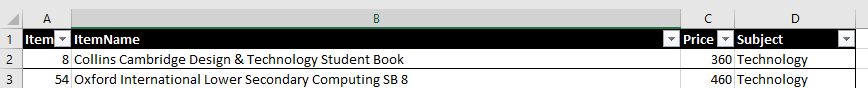
Notice that the data that does not match what you have ticked off in the list of items is hidden – the row headers turn blue as only the rows for the filtered data are shown. Also, the header of the filtered column has a small icon of a filter (at the bottom-left of the filter button) indicating that the column has a filter applied to it.
Search for Text
You can also search for specific text to filter on.
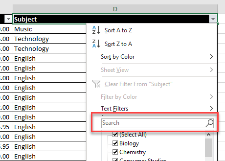
Start typing in the word you wish to filter on to limit the list below to those items.
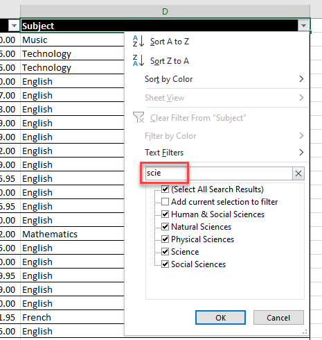
You can then click each checkbox of the items you wish to filter on.
Custom AutoFilter
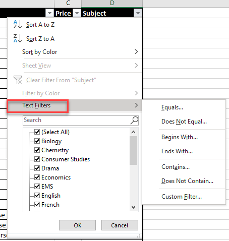
Click on the arrow next to the header column of the data you wish to filter, and then click Text Filters.
- Click on the drop-down arrow next to the header column of the data you wish to filter, and then click Text Filters.
- Choose contains… from the first drop down, and then type a word into the second drop down, e.g., Science. This filter for any rows where the text contains “science” (not case sensitive).
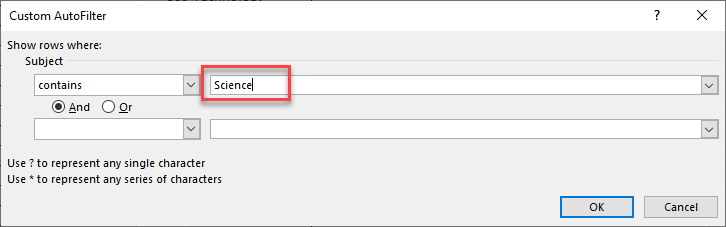
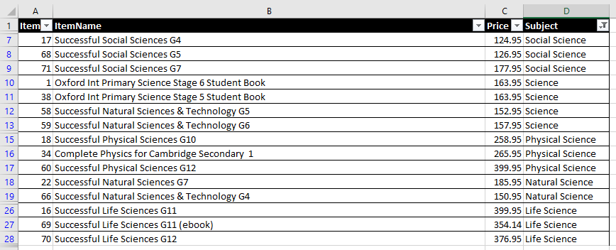
- Click OK to filter the data.
- Optionally, filter for two values in a column. Again, click on the arrow next to the header column of the data you wish to filter, and then click Text Filters. In the Custom Autofilter window (see Step 2),
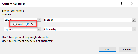
- Choose equals… from the list shown, and then choose the text you want to filter for from the drop down on the right side.
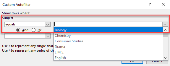
- Then click Or and type in, or choose from the list, the second value to include in the filter.
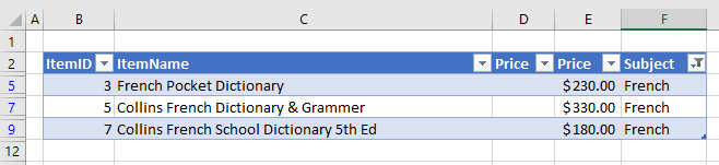
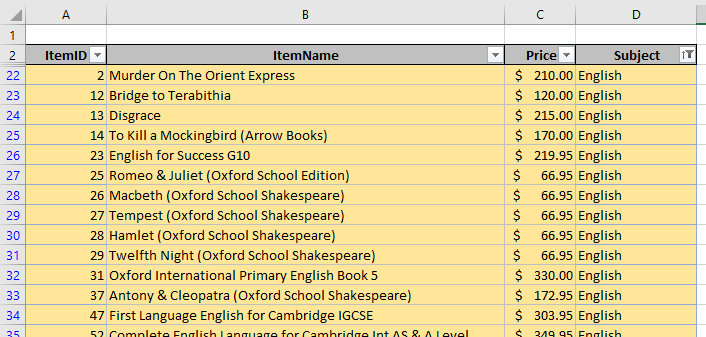
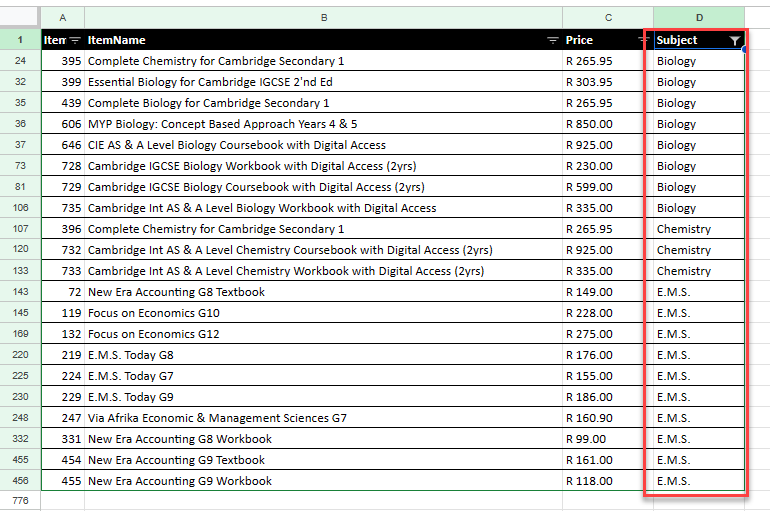
The custom filter sown below (Subject equals Biology Or equals Chemistry) tells Excel to filter out all values from the table unless the Subject is either Biology or Chemistry.
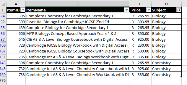
- Click OK to filter the data for both values: Biology and Chemistry.
Number Filters
Filtering numbers is similar to filtering values.
Built-in Filters
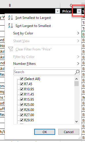
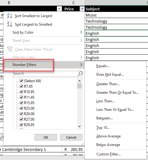
- Click the Price filter button to show the quick menu.
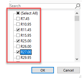
- Click Select All to remove the check mark from all the values, and then tick the checkboxes for the values you want. Click OK to filter the data.
- Or click Number Filters for a list of built-in filters settings.
- Click Above Average to show only values about the total average value of the data.
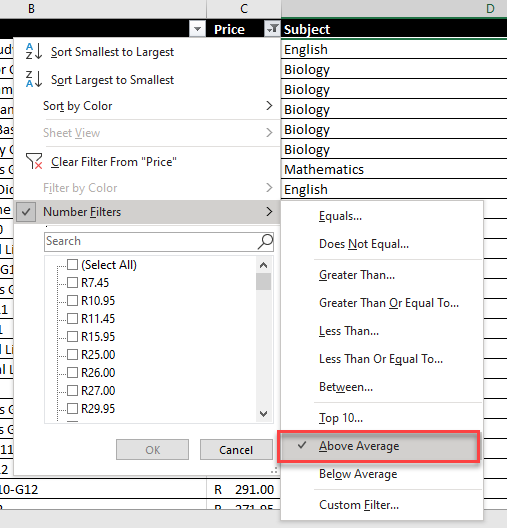
- The list is automatically filtered to reflect the filter chosen. Here, rows with values above the average Price are shown and the rest are hidden.
Custom Filters
As you do when you filter text values, you can customize number filters.
- Click on the arrow next to the header column of the data you wish to filter, and then go to Number Filters > Custom Filter… This brings up the Custom Autofilter window.
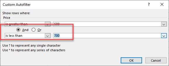
- For this example, you want to display rows where Price is between 500 and 700. For the top two fields, choose is greater than and type in 500 (the minimum value).
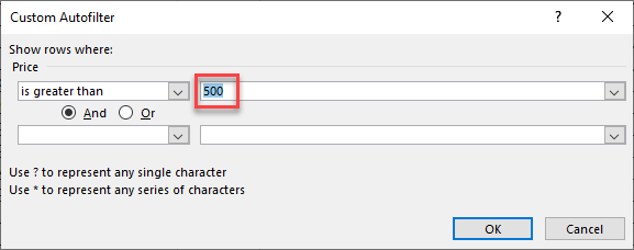
- For the lower two fields, choose is less than and type in 700 (the maximum value). Make sure the radio button is set to And.
(The settings for filtering a range between two values are: is greater than And is less than.)
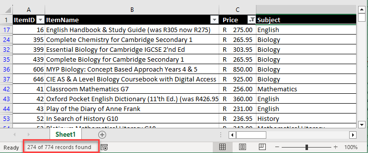
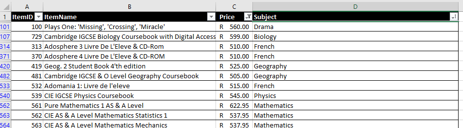
- Click OK to filter the data. Note that all rows displayed in the picture below have Prices between 500 and 700.
Filter by Color
If you have formatted your data by color, Excel has the ability to filter the data based on the colors applied.
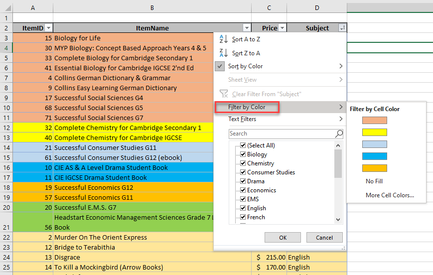
- In the filter drop down, go to Filter by Color.
- Click More Cell Colors… to see all the cell colors applied to the data.
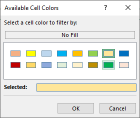
- Choose the color you wish to filter on. Preview the color in the Selected: box at the bottom. Click OK.
Clear Filter
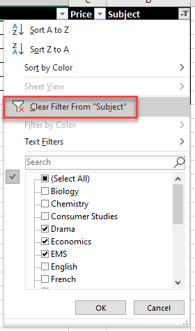
To reset your data and clear the column filter, click on the small filter to activate the drop down. Go to Clear Filter From “Subject“ to show all of that column’s data.
Another option is to tick Select All and then click OK to clear the column filter.
Clear All Filters
Above are two ways to clear filters from a single column, but if there are filters on multiple columns, you can clear them all at once instead.
▸ In the Ribbon, go to Home > Editing > Filter > Clear.
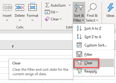
This clears the filter(s) from the entire range, but the filter headers remain at the top of each column. Everything is now visible, and the table is still ready to filter again.
Remove Filters
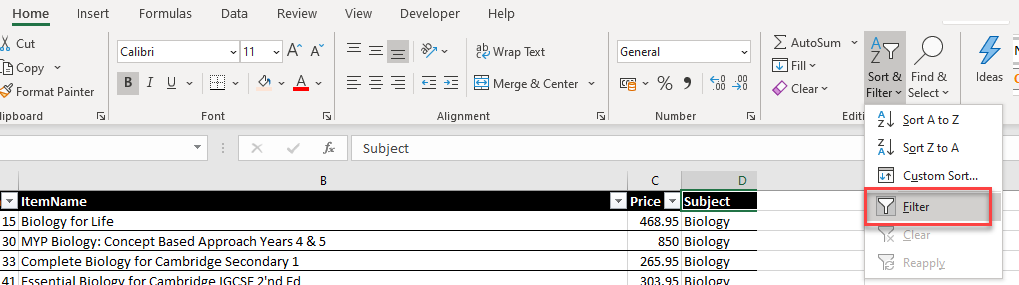
To remove the filters from the data, in the Ribbon, go to Home > Editing > Sort & Filter and then click on Filter once again. This is a toggle button; it either applies or removes filters.
Apply Multiple Filters
When your data has multiple columns, each column has a filter arrow so you can apply filters to more than one column.
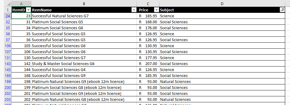
- Start with a filtered dataset. Here, Subject is filtered for Science.

- Then choose a different column to filter on. For example, filter to display only the highest values in the Price column.
- From the arrow next to Price in C1, go to Number Filters > Top 10…
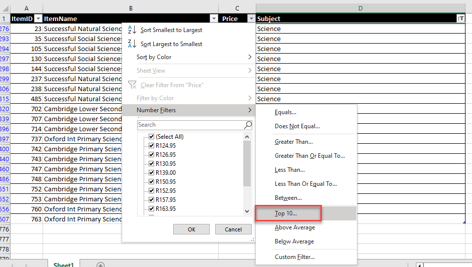
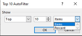
- Type in (or use the spin button to get to) how many items to filter (10, 20, etc.). For this example, choose 10 Items. Click OK.
(You could also choose to show the largest 10th percent of values instead.)
This adds a filter to the Price column while there is already a filter on the Subject column; the table has multiple filters.
Advanced Filter
Advanced Filter works differently from standard filtering. You type the filter criteria into a separate table, and then use that criteria table to filter your data (either where it stands or to a different location in the file).
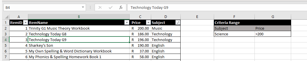
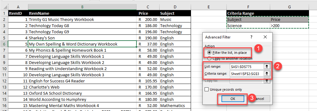
To filter data on multiple columns with an AND scenario, set up a criteria table for the data filter. In the graphic below, you wish to find all items where the Subject is Science and the Price is greater than 200. To extract all the Price values greater than 200, use a comparison operator, e.g., the greater than sign.
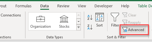
- In the Ribbon, go to Data > Sort & Filter > Advanced Filter. If the current selected cell is in the table, Excel automatically selects the entire range.
- Tick Filter the list, in-place. Set the List range (if a change is necessary) and the Criteria range.
- Then, click OK to filter the data.
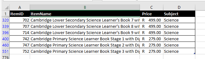
The result looks just like it would with an autofilter. You won’t see filter arrows at the top of each column, but as shown in the picture below, you can that the data is filtered by the color of the row numbers (e.g., blue 320).
Tip: Other comparison operators that are available to use are:
- Less than (<)
- Less than or Equal to (<=)
- Greater than or Equal to (>=)
- Equal to (=)
- Not Equal to (<>)
Sort Filtered Data
Filter arrows make it easy to sort the filtered data.
- First, apply filters to your data.
- Then, filter your data to show only those values you want to display.
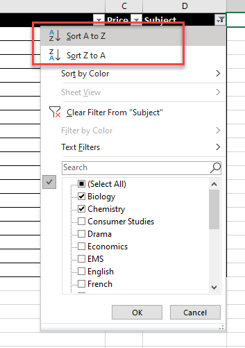
- Next, in the filter drop down, click Sort A to Z or Sort Z to A, depending on how you wish to sort the filtered data.
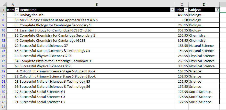
The data that is filtered is sorted. Notice a small arrow appearing next to the filter, indicating that the filtered data is sorted.
Tips for Sorted Filter
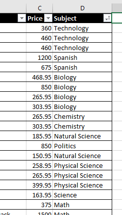
If you remove the filter, you can see that the rest of the data in the list has not been sorted.
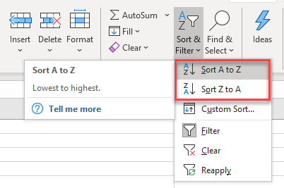
To sort the entire list of data, once the filter is cleared, you can click Sort A to Z or Sort Z to A in the filter drop down (or through the Ribbon with Home > Editing > Sort & Filter).
Filter Excel-Formatted Tables
Once you have a list of data stored in Excel, you can choose to format the data as an Excel table. Doing this automatically adds filters to the columns in the table.
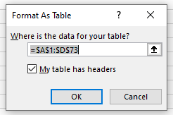
- Click in the data, and then in the Ribbon, go to Home > Styles > Format as Table. Choose a format to apply.
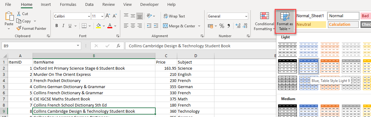
- In the Format As Table dialog box, check My table has headers (if it isn’t checked already).
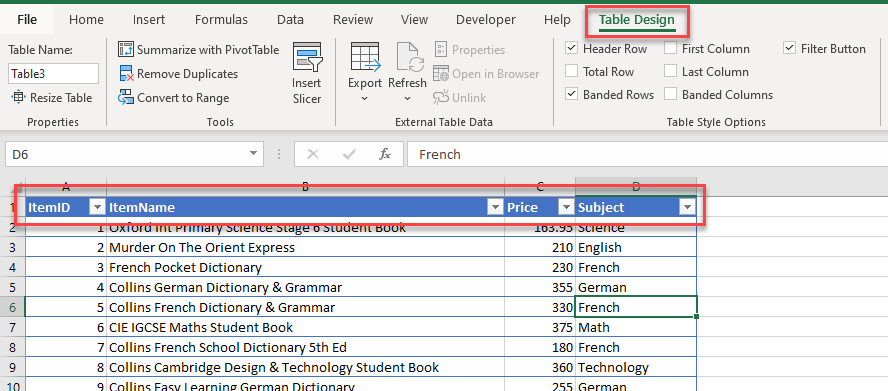
The format is applied to the data. Note that a new tab called Table Design appears in your Ribbon.
Filter Rows in Google Sheets
The processes for filtering data in Google Sheets and Excel are similar. The main difference is how items are selected from the list.
Create a Filter
In the Menu, go to Data > Create a Filter.
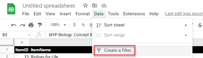
This applies small filter arrows to each column of your data.
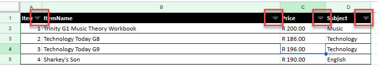
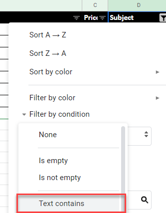
Filter for Specific Text
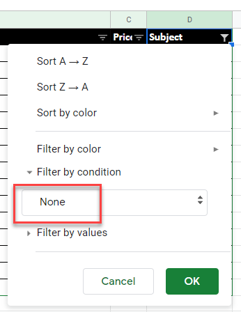
- To filter the data by specific text, click Filter by condition and then in the drop down below, choose Text contains. There are multiple conditions you can filter with.
- Type in the text to filter for, and then click OK.
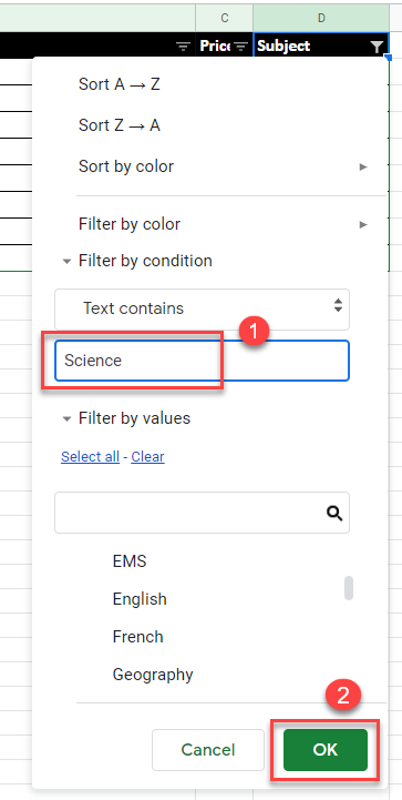
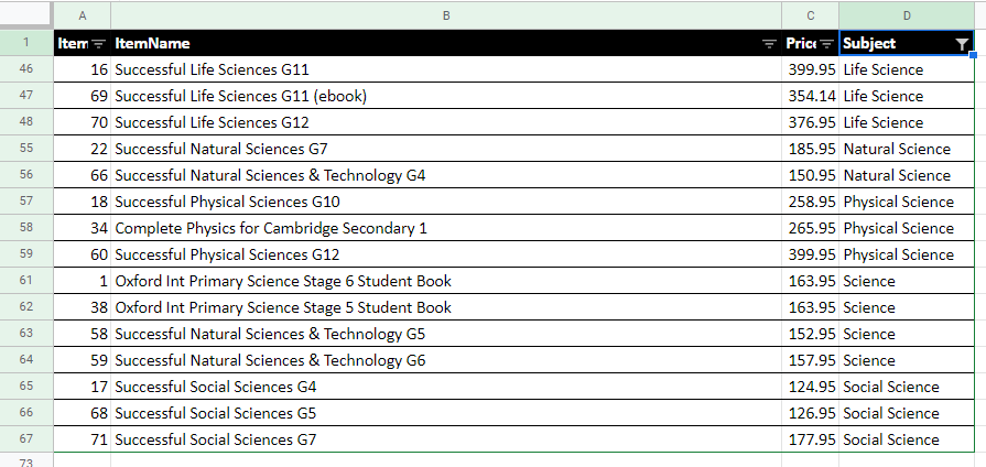
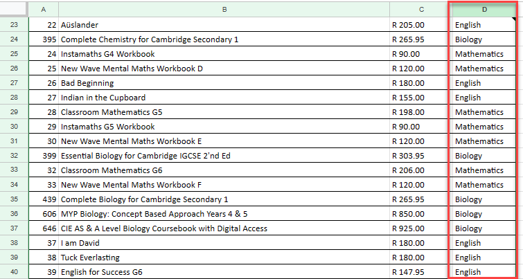
The table displays only those rows containing the relevant data.
Once you have filtered the data, you can also sort the data as you can in Excel.
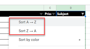
In the filter drop down, click Sort A to Z or Sort Z to A, depending on how you wish to sort the filtered data.
Note that, as with Excel, this only sorts the filtered data – not the entire data list.
To clear the filter, go to Filter by condition > None in filter the drop down, and then click OK.
Filter Values
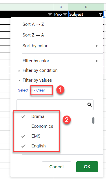
- Click on the filter arrow in the column you wish to filter on, and then, to remove the checkmarks from all values, click Clear.
Note: This works similarly to removing the checkmark from the Select All checkbox in the Excel filter menu. - Once you have cleared the checkmarks from the list of items, tick the item(s) to filter for from the list.
- Click OK to filter the data.
Tip: Using the search box with a Google Sheets filter? Don’t forget to Clear first. (This step is unnecessary in Excel.)
Filter by Color
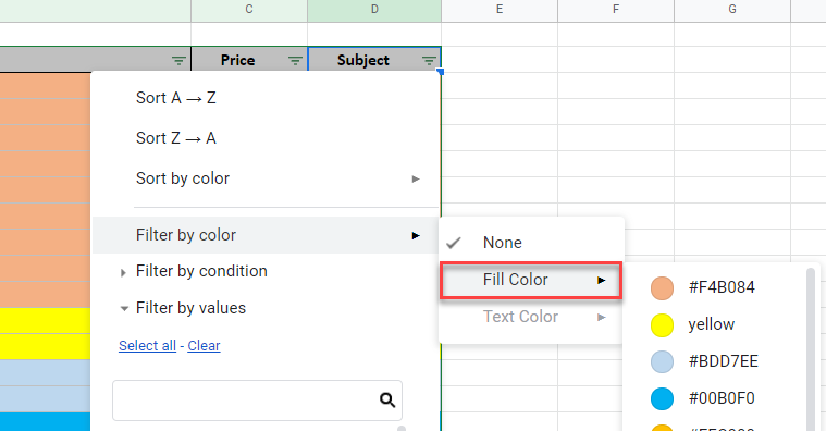
▸ From the filter drop down, go to Filter by color > Fill color and then choose one of the fill colors shown.
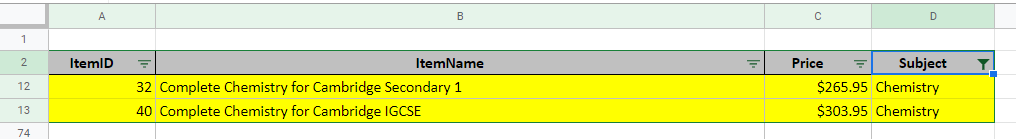
The data is filtered by the chosen color.
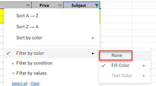
To remove just the color filter, go to Filter by color > None from the filter drop down.
Clear Filter
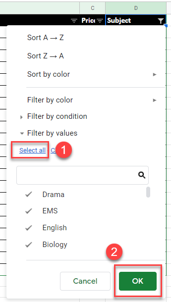
▸ To remove all filters from a column, in the drop down, click Select All and then click OK.
The filter is cleared but the filter arrows still show on the column headers.
Remove Filters
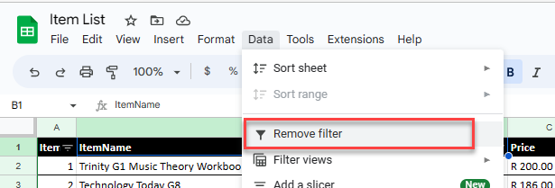
▸ To turn filtering off for all data, in the Menu, go to Data > Remove filter.
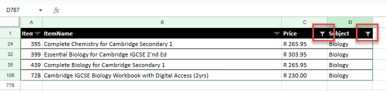
Apply Multiple Filters
Multiple filters work the same way in Google Sheets as they do in Excel. First, select one column and create your filter, and then, create a second filter by clicking the filter arrow on a second column.
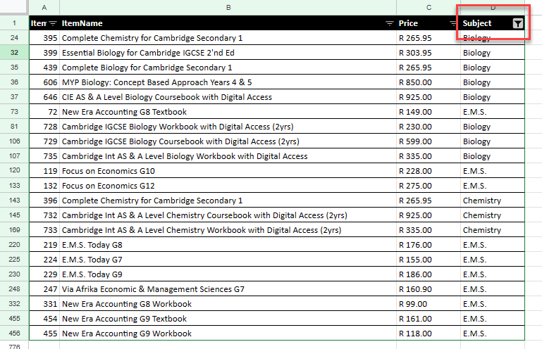
Sort Filtered Data
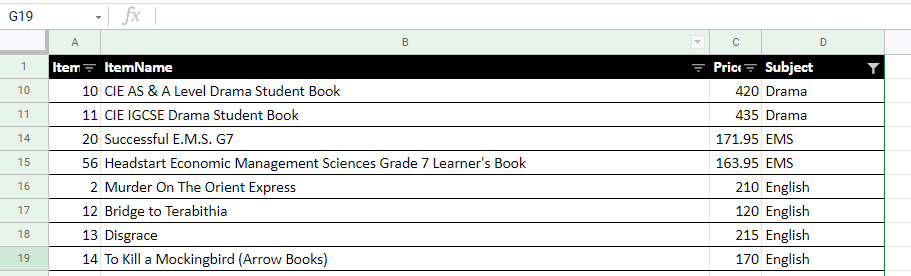
Start with filtered data, such as that shown in the picture below.
▸ Then, from the filter drop down, choose Sort A→Z.
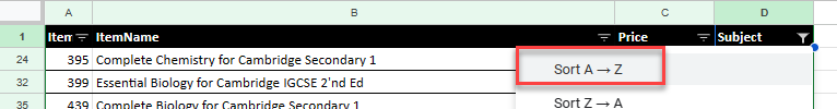
The filtered list is then sorted alphabetically.
However, if you remove the filter, you can see that the entire list has not been sorted; only the filtered data was affected by the sort.
More Tutorials on Using Filters
